Notes. Statistical consulting is like a final exam on steroids.

Transcription

1 Notes Statistical consulting is like a final exam on steroids. A statistical consultant usually works as part of a team on a project and provides statistical knowledge for the team. That team may comprise just the consultant and client, or it may include multiple members who bring overlapping expertise to the team. The consultants contribution may include problem formulation, designs for data collectiona and analysis, and writing a report that describes methods, results, and conclusions. Typically, conclusions are produced by the team after the statistical consultant discusses results with everyone. Example: OAB, overactive-bladder syndrome. Overactive Bladder Syndrome is an urological condition that sometimes is treated by lifestyle changes, sometimes by drugs, depending on the physician s evaluation and severity of patient symptoms. This project involved two pharmaceutical companies and was initiated by an independent urologist. In addition to the statistical consultant, he team for this project included two urologists from the phama companies, a statistician from one of the pharma companies who was responsible for providing data, the vice president for the urology section of one of the pharma companies. The basic question for this project was to investigate why some patients in clinical trials who received a placebo respond as well as patients who received the drug treatment but others on a placebo responded poorly. Methods involved classification and regression modeling that included variable selection and prediction. Example. A project may involve only obtaining summaries of data. A large organization that provides enhanced training for Advanced Placement classes and teachers wanted to compare test scores of students in these courses. These comparisons were to be made across school districts, schools, and teachers. Here are some questions that arose. What should be the basis for comparisons? Means? Medians? Something else? Would a difference between two districts (or schools, or teachers) indicate that one district is better than the other? Example. A company that sells medical supplies to physicians, clinics, and hospitals is audited by the State Comptroller s office for sales tax paid. Instead of conducting a complete audit of all invoices over the three-year audit period, sample-based auditing was used. Invoices from eight randomly selected days from the audit period were examined by the auditor. Total sales tax error in these invoices was dividied by total invoice amount. This ratio was multiplied by the total invoice amount for the three-year audit period to give the estimated total sales tax error. This turned out to be $700,000. Sales tax errors can occur several different ways. Supplies for Medicare/Medicaid use are not subject to state sales tax, but most customers of this company have both Medicare and non-medicare patients. Some physicians have multiple offices whose locations may have different sales tax rates. Does the method used by the auditor give a proper estimate? If not, what is the appropriate method? How accurate is a proper estimate based on this data? 1

2 Example. The Village Creek sewage treatment plant is located on the Trinity River just west of the Tarrant-Dallas county line. Water is discharged after treatment into the Trinity. During summer months when we have little rain, as much as 90% of the Trinity s flow comes from Village Creek. Chlorine used during treatment was part of the effluent discharged into the river. This chlorine is toxic to aquatic insects downstream of Village Creek. These insects are at the bottom of a food chain that includes fish, birds, and people. Under the Clean Water Act, Village Creek was required to dechlorinate its effluent before discharge. How can we assess the effect of dechlorination on the receiving stream? The CWA requires that discharge does no harm. Has this requirement been met? Whole Effluent Toxicity Tests form the basis for permitting in this situation. As these examples show, the statistician often works with people and data from unfamiliar fields. He/she must be able to learn enough about these areas for intelligent discussion with experts in those fields. The statistician may not know details about the appropriate statistical methods for the problem, but he/she must be able to follow the proper path that leads to those methods, then learn all the details and pitfalls associated with their application. The statistical consultant must: 1. understand and define the problem in statistical terms; 2. assess overall objectives and identify potential problems; 3. plan for data collection; 4. check data for errors or inconsistencies (never assume data is correct); 5. determine and implement appropriate statistical methods; 6. check, then recheck, and recheck again all code and programs used for the analysis; 7. perform analyses, check assumptions, deal with problems, recheck code; 8. discuss preliminary results, add any additional analyses; make changes to code; 9. check code and rerun, if necessary; 10. write final report. Tools. R for statistical analyses and graphics. It s free, it s widely used and accepted in many fields, it has an extensive set of addon packages that keeps R state-of-the-art, and it has unmatched graphical capabilities. Downside: it has a steep learning curve, errors in code can be subtle and difficult to identify. 2

3 Reports: PDF is the most commonly used format for reports. Printed copies are no longer needed, so graphics should make extensive use of color. PDF files can be generated by L A TEXand is strongly recommended if any mathematical notation is included. If Word is used, then a PDF version of the report is what should be delivered, not the Word document. This ensures the report can be viewed across all operating systems and devices including tablets. Presentation: PowerPoint and Keystone (mac) are most common, but latex-based beamer is useful if the presentation includes mathematical notation. Contributed library xtable provides an interface between L A TEXand output of R tables and matrices. beamer also includes navigation links to move easily among different sections of the presentation. 3

4 Case study: Johannes Kepler and his third law of planetary motion. Johannes Kepler ( ) was a mathematician who derived the fundamental laws of planetary motion that were the basis for the theory of gravity presented by Isaac Newton in Kepler was employed by a Danish nobleman, Tycho Brahe, to analyze the extensive, and very accurate for its time, sets of planetary positions. Kepler tried to fit various models to the positions of Mars but was unsuccessful until he tried fitting an ellipse. He found a near-perfect fit and this became his first law of planetary motion: all planets move in ellipses, with the sun at one focus. His second law, planets sweep out equal areas in equal times was derived from the observation that a planet moves faster when it is closer to the sun and geometrical properties of ellipses. What is remarkable about these laws is that they were derived from data obtained before telescopes were invented. At that time distances of planets from the Sun only could be obtained relative to the earth s distance from the sun, referred to as an astronomical unit (a.u.). Kepler s third law relates distance of a planet from the sun and its orbital period. He originally stated his third law as: a planet s period is proportional to the square of its distance from the Sun. Here are distances and orbital periods of the planets known to Kepler. Distance is given in a.u. and period is given in Earth years. Planet Period Distance Mercury Venus Earth 1 1 Mars Jupiter Saturn

5 Kepler s original model can be fit in R by: Planets0 = read.table(" header=true,sep=",", row.names=1) png("planets1.png",width=600,height=600) Pnames = dimnames(planets0)[[1]] tpos = rep(c(4,2),3) plot(period ~ Distance,data=Planets0,pch=19,xlab="Distance (a.u.)") title("orbital Period vs Distance for Planets Known to Kepler") text(planets0$distance, Planets0$Period, Pnames, pos=tpos,cex=.8) graphics.off() 5

6 #Kepler first hypothesized that Period is proportional to Distance squared Period = Planets0$Period Distance2 = Planets0$Distance^2 P2.lm = lm(period ~ Distance2-1) #note that this is a no-intercept model print(summary(p2.lm)) png("planets2.png",width=600,height=600) plot(period ~ Distance,data=Planets0,pch=19,xlab="Distance (a.u.)") D2 = seq(min(planets0$distance),max(planets0$distance),length=200) D2new = data.frame(distance2=d2^2) P2.pred = predict(p2.lm,newdata=d2new) lines(d2,p2.pred,col="red") text(planets0$distance, Planets0$Period, Pnames, pos=tpos,cex=.8) title("orbital Period vs Distance for Planets Known to Kepler\nwith Kepler s Original Third Law") title(sub="model: period of a planet is proportional to square of its distance",cex=.9) graphics.off() #diagnostic plots png("planets3.png",width=600,height=600) par(mfrow=c(2,2)) plot(p2.lm) mtext("diagnostic Plots for Kepler s Original Third Law", outer=true,line=-2) graphics.off() The result of this model fit is given here: Call: lm(formula = Period ~ Distance2-1) Coefficients: Estimate Std. Error t value Pr(> t ) Distance e-06 *** Residual standard error: on 5 degrees of freedom Multiple R-squared: 0.989,Adjusted R-squared: F-statistic: on 1 and 5 DF, p-value: 4.356e-06 6

7 7

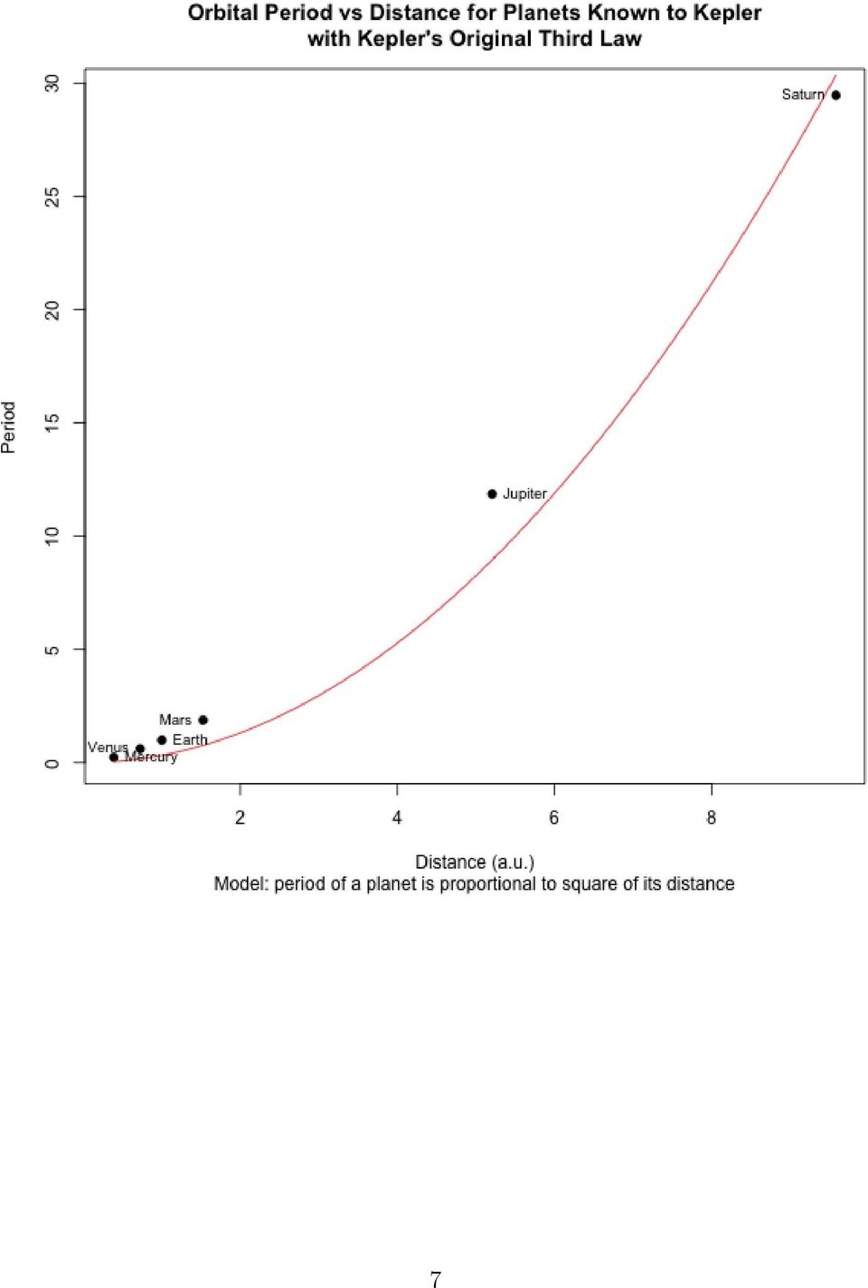
8 Kepler s original third law looks really bad. This model is an example of a power law. Power laws are fit best by log-log transformations. In R this is accomplished by #now consider log-log transformation logperiod = log(planets0$period) logdistance = log(planets0$distance) logp.lm = lm(logperiod ~ logdistance) #this model includes intercept print(summary(logp.lm)) png("planets4.png",width=600,height=600) par(mfrow=c(2,2)) 8

9 plot(logp.lm) mtext("diagnostic Plots for log-log Transformed Data", outer=true,line=-2) graphics.off() png("planets5.png",width=600,height=600) plot(logperiod ~ logdistance,pch=19) LD2 = seq(min(logdistance),max(logdistance),length=200) LD2new = data.frame(logdistance=ld2) LP2.pred = predict(logp.lm,newdata=ld2new) lines(ld2,lp2.pred,col="red") text(logdistance,logperiod,pnames,pos=tpos,cex=.9) title("orbital Period vs Distance for Planets Known to Kepler\nlog-log transformed") graphics.off() Here are the results of this fit: Call: lm(formula = logperiod ~ logdistance) Coefficients: Estimate Std. Error t value Pr(> t ) (Intercept) logdistance e-13 *** Residual standard error: on 4 degrees of freedom Multiple R-squared: 1,Adjusted R-squared: 1 F-statistic: 4.35e+06 on 1 and 4 DF, p-value: 3.17e-13 9

10 10

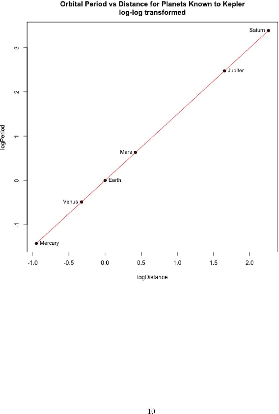
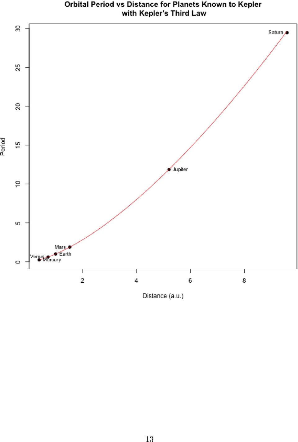
11 This analysis shows that log(period) is related to 1.5*log(Distance). In terms of the original variables, that relationship can be expressed as Period squared is proportional to Distance cubed. This implies that T 2 a 3, is constant for all planets, where T is the orbital period and a is the length of the semi-major axis of the planet (distance from the sun). Although least squares was unknown in Kepler s time, he was not satisfied with his original formulation and changed it to this new version. Here is code to produce plots that show how his third law fits the data. # plot Kepler s third law 11

12 png("planets6.png",width=600,height=600) plot(period ~ Distance,data=Planets0,pch=19,xlab="Distance (a.u.)") title("orbital Period vs Distance for Planets Known to Kepler\n with Kepler s Third Law") P2 = D2^1.5 lines(d2,p2,col="red") text(planets0$distance, Planets0$Period, Pnames, pos=tpos,cex=.8) graphics.off() ### now use new data Planets = read.table(" header=true,sep=",", row.names=1) png("planets7.png",width=600,height=900) par(mfrow=c(2,1),mar=c(1,4,3,2),oma=c(3,0,0,0)) ndx = 10:14 D2 = seq(0,max(planets$distance),length=200) P2 = D2^1.5 plot(period ~ Distance,data=Planets[-ndx,],pch=19, xlab="distance (a.u.)",xlim=c(0,1.1*max(planets$distance[-ndx]))) title("orbital Period vs Distance\nPlanets, Minor Planets, Asteroids with Kepler s Third Law") lines(d2,p2,col="red") Pnames1 = dimnames(planets)[[1]][-ndx] tpos = rep(4,length(pnames1)) names(tpos) = Pnames1 tpos["apophis"] = 2 text(planets$distance[-ndx],planets$period[-ndx],pnames1,pos=tpos) ### plot(period ~ Distance,data=Planets,pch=19,xlab="Distance (a.u.)") lines(d2,p2,col="red") text(planets$distance[ndx],planets$period[ndx], dimnames(planets)[[1]][ndx],pos=2) mtext("distance (a.u.)",outer=true,side=1,line=1.5,font=2,cex=1.2) graphics.off() 12

13 13

14 14

15 Power function of two-sample t-test The power function of the classical two-sample t-test is easy to obtain under the assumption of equal variances of the two populations. Assumptions: X and Y are independent random samples of sizes n and m, respectively, from normally distributed populations with means µ 1, µ 2 and the same s.d. σ. The one-sided hypotheses H 0 : µ 1 µ 2 H 1 : µ 1 > µ 2 are described here. Power functions for other hypotheses are derived similarly. The pooled-variance test statistic is X Y s p 1 n + 1 m, where s 2 p is the pooled variance estimator, s 2 p = 1 [ (Xi X) 2 + (Y j Y ) 2]. n + m 2 Statistical theory shows that under the null hypothesis µ 1 = µ 2, this test statistic has a t-distribution with n+m-2 d.f. Denote the critical value for a size α test with d.f. d by t d,α. In R this is obtained by qt(1-alpha,n+m-2) Therefore, the power function of this test is given by where π(δ, n, m) = P (T t d,α ), δ = µ 1 µ 2, T has a non-central t-distribution with d d.f. and non-centrality parameter λ = δ σ 1 n + 1 m, and σ is the common population s.d. In R this can be obtained with the function power.t.test() if the sample sizes are equal. This power function also can be used to obtain observable differences and sample sizes. Observable difference for this test is the value of δ such that π(δ, n, m) = 1 β. 15

16 where β is the specified probability of making a Type II error with given sample sizes n,m. That is, we want to find the difference between population means that would result in probability 1 β of rejecting the null hypothesis. Sample size determination is the same except that δ is specified and we need to find values for n,m that give required power. Suppose for example we have random samples each of size 15 and wish to determine what difference between means is detectable by a size 0.05 test with power In R this is obtained by power.t.test(n=15,power=.9,type="two.sample",alternative="one.sided") The value that is returned represents the observable difference in terms of the pooled variance. In this case that value is This implies that with independent random samples each of size 15, the means must be at least times the common s.d. for a size 0.05 test to reject with 90% probability. Suppose instead that we plan to use equal sample sizes for the two groups and need to find the sample size such that power of a size 0.05 test has power 0.90 when δ =.5σ. In R this is obtained by power.t.test(delta =.5,power=.9,type="two.sample",alternative="one.sided") The result here is n=69. If we want to obtain observable difference when the group sample sizes are not equal, then we need to input an appropriate range of values for delta into the non-central t-distribution function and then find the value of delta that gives the target for power. For example, suppose the sample sizes are 20,30 and we want to find observable difference for alpha = 0.05 and beta = n = c(20,30) df = sum(n)-2 alpha =.05 beta =.10 delta = seq(.1,.9,length=81) cv = qt(1-alpha,sum(n)-2) lambda = delta/sqrt(sum(1/n)) pwr = 1 - pt(cv,df,lambda) if(max(pwr) < 1-beta min(pwr) > 1 - beta) { cat("no values of delta gave required power\n") obsdiff = NA } else { ndx = seq(pwr)[pwr >= 1 - beta] obsdiff = delta[min(ndx)] } obsdiff 16

17 The value returned by this is obsdiff = In practice, we never use the pooled-sample t-test because Welch s approximation works well when the population variances are unequal and performs about the same as the pooled sample test when the population variances are equal. However, obtaining the power function for this test is more complicated. Let V 1 = σ2 1 n, V 2 = σ2 2 m, ˆV 1 = s2 1 n, ˆV2 = s2 2 m. Welch s approximation is based on the result: (X Y ) (µ 1 µ 2 ) V1 + V 2 t d, where degrees of freedom is given by d = (V 1 + V 2 ) 2. V1 2 + V 2 2 n 1 m 1 In practice we replace V i by its estimate ˆV i to obtain d.f. The power function for a size alpha test is then π w (δ, n, m) = 1 pt(cv, d, λ ), where the non-centrality parameter is given by λ = To simplify, let Then and d.f. is δ V1 + V 2. a = σ2 2, b = m σ1 2 n. λ = δ nb σ 1 a + b d = (a + b)2 b 2 + a2 n 1 bn 1 In practice we estimate a by â = s2 2. s 2 1 Here is a simple R function that evaluates this power function. 17

18 power.welch.test = function(delta,n1,sig1,a,b,alpha=.05) { # n1 is sample size of group 1 # b = n2/n1 # sig1 is sd of group 1 # a = (sig2/sig1)^2 # either delta or n1 can be a vector but not both df = (a+b)^2/(b^2/(n1-1) + a^2/(b*n1-1)) lambda = delta*sqrt(n1*b/(a+b))/sig1 cv = qt(1-alpha,df) pwr = 1 - pt(cv,df,lambda) pwr } As a test, this function with n1=20, a=1, b=1.5 should give the same result as the equal variance power function. Scripts Links to scripts used in class are here