Chapter 1: Looking at Data Section 1.1: Displaying Distributions with Graphs

Transcription

1 Types of Variables Chapter 1: Looking at Data Section 1.1: Displaying Distributions with Graphs Quantitative (numerical)variables: take numerical values for which arithmetic operations make sense (addition/averaging) Categorical variables: place an individual into one of several groups or categories data. Example Identify whether the following questions would give you categorical or quantitative a.) What letter grade did you get in your Calculus class last semester? b.) How long does it take you to walk to class from your dorm/apartment? c.) Do you like Starbucks? Distribution of Variables The distribution of a variable describes the values the variable takes and how often it takes each value. If you have more than one variable in your problem, you should look at each variable by itself before you look at relationships between the variables.

2 Always start by displaying the variables graphically before you do any other statistical analysis. What kind of graph should we use? Start by identifying the type of variable we are graphing Categorical or Quantitative. If Categorical 1.) Bar Graphs 2.) Pie Charts In a poll of 200 parents of children ages 6 12, respondents were asked to name the most disgusting thing ever found in their children s rooms. The results are below (J&C, 2005) Most disgusting thing # of parents % of parents Food related % Animal and insect related nuisances 22 11% Clothing (dirty socks and underwear especially) 22 11% Other 50 25% Bar Graph (can use either # of parents or % of parents): Typically with bar graphs, the y axis represents the frequency (# of observations) in the categories. Units can give multiple answers or no answer. Pie Chart: Percents must add to 100%. Each unit must give only one answer % animal type of disgusting mess animal clothing food other % other 11.0% clothing Count % food 20 0 animal clothing food other type of disgusting mess Cases weighted by # of parents Cases weighted by # of parents

3 If Quantitative 1.) Stem and leaf plots a. Displays actual values of all observations b. Good for small amounts of data 2.) Histograms a. Displays only summary information b. Used for large amounts of data Steps for Creating Stem and Leaf plots: 1. Put data in numerical order from smallest to largest. 2. Separate each observation into a stem and a leaf (Note: leaf = final digit, stem = remaining digits. In the case of a single digit number like 7, use 07 so that 0 is the stem.) 3. Write stem numbers in order in a vertical column with the smallest at the top. Do not skip numbers. Draw a vertical line next to the stem. 4. Write each leaf in the row to the right of its stem, in increasing order out from the stem. Show each numerical value as many times as it appears in the dataset. 5. It is possible to trim any digits that you feel may be unnecessary. You can document that the numbers shown are thousands, for example, if you trim off the last three digits. Example. You investigate the amount of time students spend online (in minutes). You study 28 students, and their times are listed below. Show the distribution of times with a stemplot Back to Back Stemplots help us compare two distributions. Write stems as usual but with a vertical line both to the left and right. Arrange leaves on each stem in increasing order extending out from the stem. Example (Con t). You now include the amount of time professors spend online(in minutes). You study 15 professors and their times are listed below. Show the distribution of times with a back toback stemplot

4 Histograms: The x axis is divided into intervals of equal width. The height of the graph over a given interval represents the count or percent of the observations in that interval. How many intervals should be used? Try not to have too many intervals containing either 0 or 1 data values. Do not use too few intervals such that you lose all of the information. Do not make the graph so detailed that it is no longer a summary. Example. How do histograms differ from bar graphs? Histograms - The variable graphed is quantitative. - The bars of each interval touch. - The graph has a continuous x-axis with values in order. Bar graphs - The variable graphed is categorical. - The bars do not touch. - The x-values can be listed in any order. If the overall pattern of a large number of observations is quite regular, we choose to describe it by a smooth curve called a density curve. A density curve is an idealized model for a distribution of data.

5 Section 1.2: Describing Distributions with Numbers Now that we have graphed the data, look at the graph and see what it tells you. Graphs show you the overall pattern of the data and any deviations from that pattern (outliers). Describing Graphs of Quantitative Variables The pattern is described by the shape, center and spread. 1.) Shape: defined by classifying the graph in two ways a. The number of peaks: i. 1= Unimodal ii. 2= Bimodal iii. 3 or more= multimodal b. The skewness of the graph: i. Symmetric: median is approximately equal to the mean ii. Right Skewed: Median<mean 1. Long tail to the right iii. Left Skewed: Median > mean 1. Long tail to the left 2.) Center: defined by the middle value or average value. a. Mode: The measurement value that occurs most often. b. Median: The middle value when the measurements are arranged from the lowest to highest. Steps to finding the median: a. Arrange observations from smallest to largest. b. Count the observations. c. Calculate n 1 to find the center of the data set 2 d. If n is odd, M is the data point at the center of the data set. e. If n is even, n 1 falls between 2 data points, called the middle pair, M = the average of the middle pair. 2 c. Mean: the sum of the measurements divided by the total number of measurements (a.k.a. average) x n ( x x... x ) n n xi

6 3.) Spread: defines the width of the distribution. a. Range: The difference between the largest and the smallest measurements of a dataset. b. Interquartile Range (IQR): the distance between the first and third quartiles. IQR Q3 Q1 (Note: IQR= 0 does not mean that there is no spread.) The quartiles Q 1 and Q 3 are calculated as follows: a. Arrange the observations in increasing order and locate the median M in the ordered list of observations. M = the 50% or 2 nd quartile. b. The 1 st quartile Q1 is the median of the observations whose position in the ordered list is to the left of the location of the overall median, M. Another name for Q1 is the 25 th percentile. c. The third quartile Q 3 is the median of the observations whose position in the ordered list is to the right of the location of the overall median. Another name for Q is the 75 th percentile. 3 c. Variance, s 2 of a set of observations is: ( x1 x) ( x2 x)... ( xn x) 1 S ( xi x) n 1 n 1 The standard deviation, s, is the square root of the variance. (Note: variance or standard deviation =0 means there is no spread) 2 Percentiles: The p th percentile of a swet of observations is the value such that p% of the observations fall at or below this number. Note: 25 th percentile = Q1 75 th percentile = Q3 Five Number Summary: gives us a brief description of the data using 5 points 1.) Minimum 2.) Q1 3.) Median 4.) Q3 5.) Maximum Outliers: an observation is considered an outlier if it falls 1.5 x IQR above the third quartile or 1.5 x IQR below the first quartile.

7 Boxplots A boxpot is a graph of the five number summary. Lines extend from the box out to the smallest and largest observations. A central box spans the quartiles Q1 to Q3. A line inside the box marks the median M. Lines extend from the box out to the smallest and largest observations. A modified boxplot has lines that extend from the box out to the smallest and larges observations which are not outliers, dots mark any outliers. Resistant Measures resist the influence of extreme observations. Best Method for determining Center and Spread: When you have a skewed distribution or a distribution with outliers, use the median and the IQR for the measures of center and spread. The mean and standard deviation are good measures of center and spread for reasonably symmetric distributions free of outliers.

8 Example. We will use this example throughout the entire lesson, so keep this page out next to your notes. 30 students were asked to give a score of how much money they spend in a week on fast food and eating out. Their answers are recorded below:

9

10 Section 1.3: The Normal Distribution Density Curves A density curve is a curve that a.) Is always on or above the horizontal axis b.) Has area exactly 1 underneath it c.) Describes the overall pattern of a distribution. The area under the density curve and above any range of values is the relative frequency of all observations that fall in that range. Physical Interpretation a.) The mean of a density curve is the point at which the curve would balance if made of solid material b.) The median of a density curve is the point that divides the area under the curve in half. The Normal Distribution There is one important class of curves that we will be working with throughout the semester called the normal curves which have the following properties: a.) They are all symmetric, bell shaped, unimodal b.) The mean and median are always sin the center of the graph (and equal) c.) The standard deviation σ controls the spread of a normal curve d.) Changing the mean μ moves the normal curve along the horizontal axis e.) The normal curve is completely determined by μ and σ. f.) The distribution is abbreviated N(μ, σ). g.) The probabilities are areas under the normal curve between the points of interest.

11 The Rule In the normal distribution with mean μ and standard deviation σ: Approximately 68% of the observations fall within σ of the mean μ. Approximately 95% of the observations fall within 2σ of μ. Approximately 99.7% of the observations fall within 3σ of μ. EXAMPLE (From Moore and McCabe fifth edition) Bigger animals tend to carry their young longer before birth. The length of horse pregnancies from conception to birth varies according to a roughly normal distribution with mean 336 days and standard deviation 3 days. Use the rule to answer the following questions. 1. Between what values do the length of the middle 68% of all horse pregnancies fall? 2. How short are the shortest 2.5% of all horse pregnancies? How long do the longest 2.5% last? 3. What percent of the horse pregnancies last between 336 and 342 days? 4. On the Normal distribution curve below, label μ, σ, 336, 342. Shade the percent calculated above.

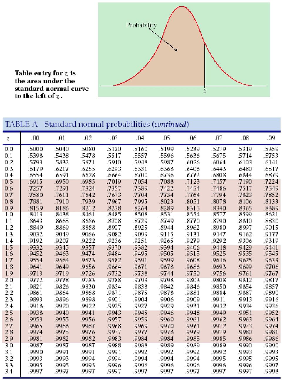
12 NORMAL DENSITY FUNCTION What if you need different probabilities for X N(μ, σ) other than the ones you can locate using the Rule? The equation for the normal density curve is: 1 e x 2 This is not an integrable function, so the standard normal table was created to find probabilities for the Standard Normal Distribution. Standard Normal Distribution has mean 0 and standard deviation 1 when you have N(0,1), you can use the Z table to find probabilities. Using the Z table: 1.) We have to have a variable with normal distribution with mean 0 and standard deviation 1. a. If we do not have a standard normal, we have to convert X N(μ, σ) to the standard normal Z N(0, 1). X i. To do this use: Z Note: Z scores tell you how far (measured in standard deviations) the original observations fall from the mean. Example. If Z N(0, 1), find the following: P(Z<2.21) = P(Z< 1.47) = P(Z>.65) = P(Z>.03) = P( Z 1.48) = P( 1.48 Z 1.48) = PZ ( 4.9) = PZ ( 5.34) =

13 Example. The height of women aged are approximately normal with mean 64 inches and standard deviation 2.7 inches. Men, the same age have mean height 69.3 inches with standard deviation 2.8 inches. What are the z scores for a woman 6 feet tall and a man 6 feet tall? What information do the z scores give that actual heights do not? ***Steps to Finding a Probability when X N(μ, σ) 1. Draw the curve and shade the area you want to find. 2. Write your probability statement in terms of X. If you have P(X > x), change to less than by using the rule P(X > x) = 1 P(X < x). X 3. Convert X to Z using Z. Set P(X < x) = P(Z < z). 4. Look up the probability for your z score on the standard normal table. The Z table gives you the probability PZ ( z). 5. If the z score is between 2 table values, either pick the closer one or average the two closest values. Example. If X N(4, 1.5), find the following probabilities using table A: a. P( X 3) = d. P(X<4)= b. P( X 4.5) = e. P(X=3.45)= c. P(3 X 4.56) = f. P(X>11)=

14 Example. In the year 2000, the score of men on the math part of the SAT approximately followed a normal distribution with mean 530 and standard deviation 112. a. What portion of the men scored above 450? b. What portion scored between 450 and 550? Now let s reverse things! When going backwards, we are given the probability and asked to find the z score. This involves using the standard normal table in a backwards fashion. Lookup the probability in the body of the table and read off the z score from the outside margin. ***Finding X when given a Probability 1. Draw the curve and shade in the area you want to find. 2. Set up your problem as follows the 1 probability rule.) P( Z z ) probability (Note: adjust to < if necessary by using 0 3. Find the z score by looking up the probability in the body of the standard normal table. x 4. Convert the z score to x using z. 5. If you have a two sided central probability, use the following rule: P( z Z z ) 2 P( Z z )

15 Example. Find z 0 for each of the following: a. P(Z < z 0 ) = b. P(Z < z 0 ) = c. P(Z > z 0 ) = d. P(Z > z 0 ) = 0.0 e. P( z 0 < Z < z 0 ) = 0.5 f. P( z 0 < Z < z 0 ) =.65 EXAMPLE A physical fitness association is including the mile run in its secondary school fitness test for boys. The time for this event for boys in secondary school is approximately normally distributed with mean of 450 seconds and standard deviation of 40 seconds. If the association wants to designate the fastest 10% as excellent, what time should the association set for this criterion?

16 ADDITIONAL PROBLEMS SECTION 1.3 Checking account balances are ~ N(1325, 25). Bill has a balance of $1270. a) What is the probability an account will have less money than Bill s? b) What is the probability an account balance will be more than $1380? c) What is the probability an account balance will be exactly $1380? d) What is the probability an account will have less than $1325 (the mean)? e) What is the probability that an account will have between $1310 and $1390? f) What is the probability an account will have less than $10?

17 g) What is the account balance, x 0, such that the percentage of balances less than it is 23%? h) What is the account balance, x 0, such that the probability of a balance being more than it is 0.15? i) What is the account balance, x, such that the probability of a balance being more than it is 0.5? (Hint: 0 you should be able to do this one without math.) j) Between what 2 central values do 40% of the balances fall?

18

19