Chapter 6 The 2 k Factorial Design. Design & Analysis of Experiments 8E 2012 Montgomery

Transcription

1 The 2 k Factorial Design 1

2 Design of Engineering Experiments Part 5 The 2 k Factorial Design Text reference, Special case of the general factorial design; k factors, all at two levels The two levels are usually called low and high (they could be either quantitative or qualitative) Very widely used in industrial experimentation Form a basic building block for other very useful experimental designs (DNA) Special (short-cut) methods for analysis We will make use of SAS 2

3 3

4 6.2 The Simplest Case: The and + denote the low and high levels of a factor, respectively Low and high are arbitrary terms Geometrically, the four runs form the corners of a square Factors can be quantitative or qualitative, although their treatment in the final model will be different 4

5 Chemical Process Example A = reactant concentration, B = catalyst amount, y = recovery 5

6 Analysis Procedure for a Factorial Design Estimate factor effects Formulate model With replication, use full model With an unreplicated design, use normal probability plots Statistical testing (ANOVA) Refine the model Analyze residuals (graphical) Interpret results 6

7 Estimation of Factor Effects A y y A ab a b (1) 2n 2n [ ab a b (1)] 1 2n B y y B ab b a (1) 2n 2n [ ab b a (1)] 1 2n ab (1) a b AB 2n 2n [ ab (1) a b] 1 2n A B See textbook, pg for manual calculations The effect estimates are: A = 8.33, B = -5.00, AB = 1.67 Practical interpretation? Design-Expert analysis 7

8 Estimation of Factor Effects Form Tentative Model Term Effect SumSqr % Contribution Model Intercept Model A Model B Model AB Error Lack Of Fit 0 0 Error P Error Lenth's ME Lenth's SME

9 Statistical Testing - ANOVA The F-test for the model source is testing the significance of the overall model; that is, is either A, B, or AB or some combination of these effects important? 9

10 Statistical Testing - ANOVA SAS Code and Output data one; input A B yield; cards; ; proc glm; class A B; model yield = A B; run; 10

11 Statistical Testing - ANOVA 11

12 Residuals and Diagnostic Checking 12

13 The Regression Model Code the levels of factor A and B as follows Fit regression model 13

14 The Regression Model SAS Code and Output data one; input A B yield; cards; ; proc reg; model yield = A B; run; 14

15 The Regression Model Analysis of Variance Sum of Mean Source DF Squares Square F Value Pr > F Model <.0001 Error Corrected Total Parameter Estimates Parameter Standard Variable DF Estimate Error t Value Pr > t Intercept <.0001 A <.0001 B

16 The Response Surface 16

17 6.3 The 2 3 Factorial Design 17

18 Effects in The 2 3 Factorial Design A y y A B y y B C y y C etc, etc,... A B C Analysis done via computer 18

19 An Example of a 2 3 Factorial Design A = gap, B = Flow, C = Power, y = Etch Rate 19

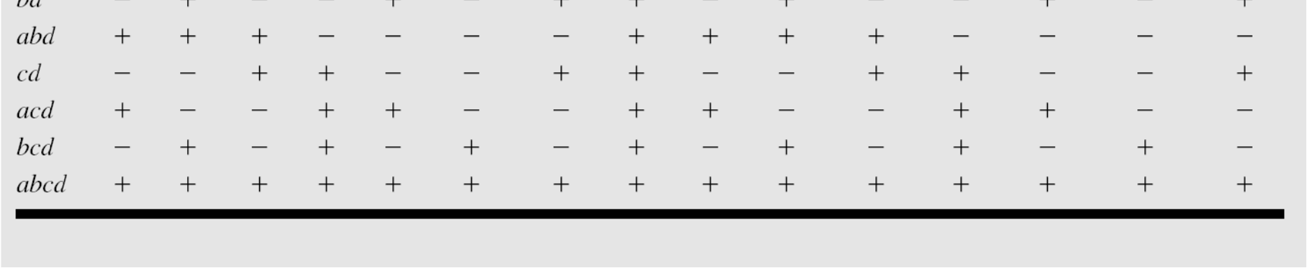
20 Table of and + Signs for the 2 3 Factorial Design (pg. 244) 20

21 Properties of the Table Except for column I, every column has an equal number of + and signs The sum of the product of signs in any two columns is zero Multiplying any column by I leaves that column unchanged (identity element) The product of any two columns yields a column in the table: A B AB 2 AB BC AB C AC Orthogonal design Orthogonality is an important property shared by all factorial designs 21

22 Estimation of Factor Effects 22

23 ANOVA Summary Full Model 23

24 Model Coefficients Full Model 24

25 Refine Model Remove Nonsignificant Factors 25

26 Model Coefficients Reduced Model 26

27 Model Summary Statistics for Reduced Model R 2 and adjusted R 2 R R 2 2 Adj 5 SSModel SS T SSE / df / SS T E 5 / dft /15 R 2 for prediction (based on PRESS) 2 PRESS RPred SS T 27

28 Model Summary Statistics Standard error of model coefficients (full model) 2 ˆ ˆ MSE se( ) V ( ) k k n2 n2 2(8) Confidence interval on model coefficients ˆ ( ˆ) ˆ ( ˆ t se t se ) /2, df /2, df E E 28

29 The Regression Model 29

30 Model Interpretation Cube plots are often useful visual displays of experimental results 30

31 Cube Plot of Ranges What do the large ranges when gap and power are at the high level tell you? 31

32 32

33 More on the 2 3 Factorial Design See p for definitions of effects See p for Other Methods for Judging the significance of Effects. 33

34 6.4 The General 2 k Factorial Design Section 6-4, pg. 253, Table 6-9, pg. 254 There will be k main effects, and k two-factor interactions 2 k three-factor interactions 3 1 k factor interaction 34

35 6.5 Unreplicated 2 k Factorial Designs These are 2 k factorial designs with one observation at each corner of the cube An unreplicated 2 k factorial design is also sometimes called a single replicate of the 2 k These designs are very widely used Risks if there is only one observation at each corner, is there a chance of unusual response observations spoiling the results? Modeling noise? 35

36 Spacing of Factor Levels in the Unreplicated 2 k Factorial Designs If the factors are spaced too closely, it increases the chances that the noise will overwhelm the signal in the data More aggressive spacing is usually best 36

37 Unreplicated 2 k Factorial Designs Lack of replication causes potential problems in statistical testing Replication admits an estimate of pure error (a better phrase is an internal estimate of error) With no replication, fitting the full model results in zero degrees of freedom for error Potential solutions to this problem Pooling high-order interactions to estimate error Normal probability plotting of effects (Daniels, 1959) Other methods see text 37

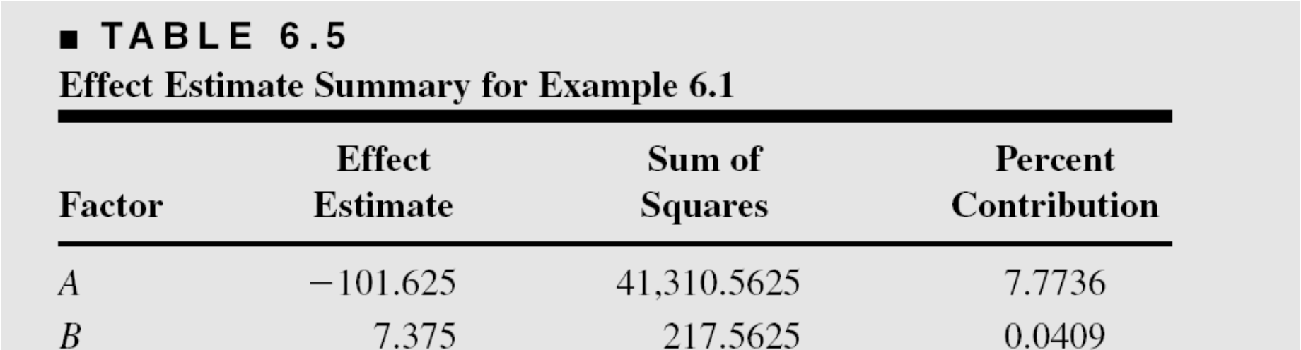
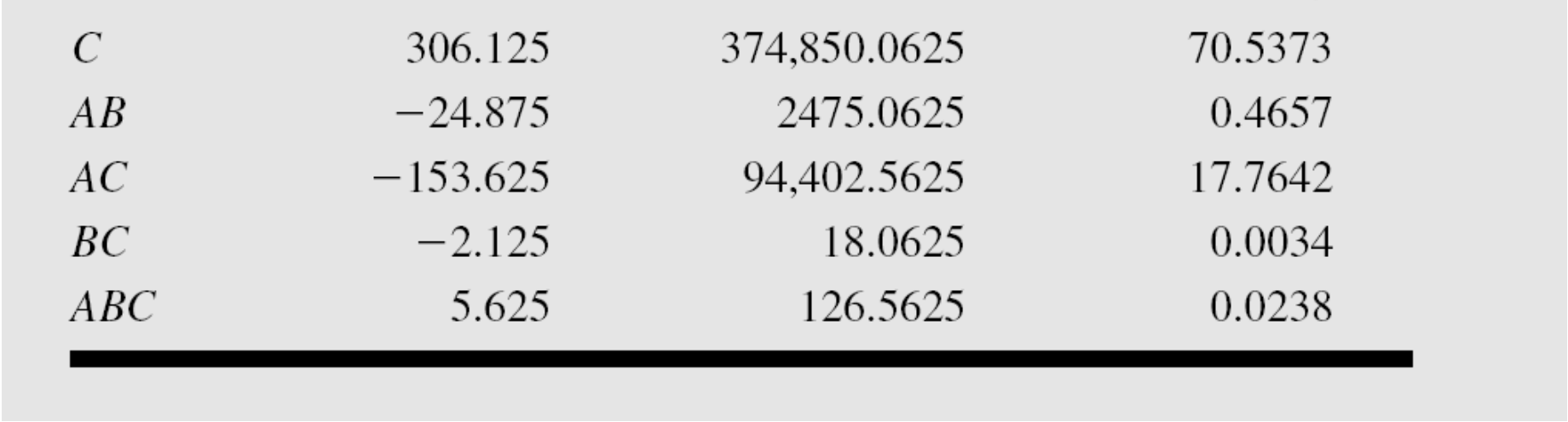
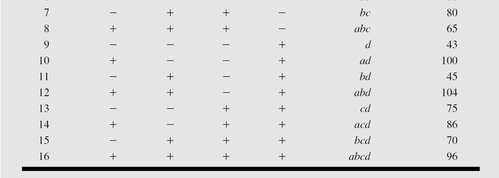
38 Example of an Unreplicated 2 k Design A 2 4 factorial was used to investigate the effects of four factors on the filtration rate of a resin The factors are A = temperature, B = pressure, C = mole ratio, D= stirring rate Experiment was performed in a pilot plant 38

39 The Resin Plant Experiment 39

40 The Resin Plant Experiment 40

41 41

42 Estimates of the Effects 42

43 The Half-Normal Probability Plot of Effects 43

44 Design Projection: ANOVA Summary for the Model as a 2 3 in Factors A, C, and D 44

45 The Regression Model 45

46 Model Residuals are Satisfactory 46

47 Model Interpretation Main Effects and Interactions 47

48 Model Interpretation Response Surface Plots With concentration at either the low or high level, high temperature and high stirring rate results in high filtration rates 48

49 Outliers: suppose that cd = 375 (instead of 75) 49

50 50

51 Dealing with Outliers Replace with an estimate Make the highest-order interaction zero In this case, estimate cd such that ABCD = 0 Analyze only the data you have Now the design isn t orthogonal Consequences? Causing significant problems in interpreting the normal probability plot. 51

52 The Drilling Experiment Example 6.3 A = drill load, B = flow, C = speed, D = type of mud, y = advance rate of the drill 52

53 Normal Probability Plot of Effects The Drilling Experiment 53

54 DESIGN-EXPERT Plot Residuals vs. Predicted adv._rate Predicted Re sid uals Residual Plots 54

55 Residual Plots The residual plots indicate that there are problems with the equality of variance assumption The usual approach to this problem is to employ a transformation on the response Power family transformations are widely used * y Transformations are typically performed to Stabilize variance Induce at least approximate normality Simplify the model y 55

56 Selecting a Transformation Empirical selection of lambda Prior (theoretical) knowledge or experience can often suggest the form of a transformation Analytical selection of lambda the Box-Cox (1964) method (simultaneously estimates the model parameters and the transformation parameter lambda) Box-Cox method implemented in Design-Expert 56

57 (15.1) 57

58 The Box-Cox Method DESIGN-EXPERT Plot adv._rate Lambda Current = 1 Best = Low C.I. = High C.I. = 0.32 Recommend transform: Log (Lambda = 0) Ln(ResidualSS) Box-Cox Plot for Power Transforms A log transformation is recommended The procedure provides a confidence interval on the transformation parameter lambda If unity is included in the confidence interval, no transformation would be needed Lambda 58

59 Effect Estimates Following the Log Transformation Three main effects are large No indication of large interaction effects What happened to the interactions? 59

60 ANOVA Following the Log Transformation 60

61 Following the Log Transformation 61

62 The Log Advance Rate Model Is the log model better? We would generally prefer a simpler model in a transformed scale to a more complicated model in the original metric What happened to the interactions? Sometimes transformations provide insight into the underlying mechanism 62

63 6.6 Other Examples of Unreplicated 2 k Designs The sidewall panel experiment (Example 6.4, pg. 271) Two factors affect the mean number of defects A third factor affects variability Residual plots were useful in identifying the dispersion effect The oxidation furnace experiment (Example 6.5, pg. 274) Replicates versus repeat (or duplicate) observations? Modeling within-run variability 63

64 Example 6.6, Credit Card Marketing, page 278 Using DOX in marketing and marketing research, a growing application Analysis is with the JMP screening platform 64

65 Other Analysis Methods for Unreplicated 2 k Designs 6.5 Lenth s method (see text, pg. 262) Analytical method for testing effects, uses an estimate of error formed by pooling small contrasts Some adjustment to the critical values in the original method can be helpful Probably most useful as a supplement to the normal probability plot Conditional inference charts (pg. 264) 65

66 Overview of Lenth s method For an individual contrast, compare to the margin of error 66

67 67

68 Adjusted multipliers for Lenth s method Suggested because the original method makes too many type I errors, especially for small designs (few contrasts) Simulation was used to find these adjusted multipliers Lenth s method is a nice supplement to the normal probability plot of effects JMP has an excellent implementation of Lenth s method in the screening platform 68

69 69

70 6.7 The 2 k design and design optimality The model parameter estimates in a 2 k design (and the effect estimates) are least squares estimates. For example, for a 2 2 design the model is y x x x x (1) ( 1) ( 1) ( 1)( 1) a (1) ( 1) (1)( 1) b ( 1) (1) ( 1)(1) ab (1) (1) (1)(1) The four observations from a 2 2 design (1) a y=xβ + ε, y 1 2, X, β, ε b ab

71 The least squares estimate of β is ˆ -1 β =(XX) Xy (1) abab aabb(1) baba(1) (1) abab (1) abab ˆ 4 0 (1) abab aabb( ˆ 1 1 a ab b (1) 1) 4 ˆ I 4 4 baba(1) 2 b ab a (1) ˆ (1) abab 4 12 (1) abab 4 The usual contrasts The XX matrix is diagonal consequences of an orthogonal design The regression coefficient estimates are exactly half of the usual effect estimates 71

72 The matrix XX has interesting and useful properties: V ˆ 2 1 ( ) (diagonal element of ( ) ) 2 4 XX Minimum possible value for a four-run design ( XX ) 256 Maximum possible value for a four-run design Notice that these results depend on both the design that you have chosen and the model What about predicting the response? 72

73 2-1 V[ yˆ ( x1, x2)] x(xx) x x [1, x, x, x x ] V[ yˆ ( x, x )] (1 x x x x ) 4 The maximum prediction variance occurs when x 1, x 1 2 V[ yˆ ( x1, x2)] The prediction variance when x is V[ yˆ ( x1, x2)] 4 What about average prediction variance over the design space? x 73

74 Average prediction variance I V yˆ x x dxdx A A [ ( 1, 2) 1 2 = area of design space = (1 x x x x ) dxdx

75 Design-Expert Software Min StdErr Mean: Max StdErr Mean: Cuboidal radius = 1 Points = FDS Graph StdErr Mean Fraction of Design Space 75

76 For the 2 2 and in general the 2 k The design produces regression model coefficients that have the smallest variances (D-optimal design) The design results in minimizing the maximum variance of the predicted response over the design space (G-optimal design) The design results in minimizing the average variance of the predicted response over the design space (Ioptimal design) 76

77 Optimal Designs These results give us some assurance that these designs are good designs in some general ways Factorial designs typically share some (most) of these properties There are excellent computer routines for finding optimal designs (JMP is outstanding) 77

78 6.8 Addition of Center Points to a 2 k Designs Based on the idea of replicating some of the runs in a factorial design Runs at the center provide an estimate of error and allow the experimenter to distinguish between two possible models: First-order model (interaction) Second-order model 0 k k k y x x x 0 i i ij i j i1 i1 ji k k k k 2 i i ij i j ii i i1 i1 ji i1 y x x x x 78

79 79

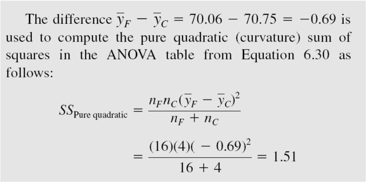
80 y F y C no "curvature" The hypotheses are: SS Pure Quad H H 0 1 k : 0 i1 k : 0 i1 ii ii nn F C( yf yc) n n This sum of squares has a single degree of freedom F C 2 80

81 Example 6.7, Pg. 286 Refer to the original experiment shown in Table Suppose that four center points are added to this experiment, and at the points x1=x2 =x3=x4=0 the four observed filtration rates were 73, 75, 66, and 69. The average of these four center points is 70.75, and the average of the 16 factorial runs is Since are very similar, we suspect that there is no strong curvature present. nc 4 Usually between 3 and 6 center points will work well Design-Expert provides the analysis, including the F-test for pure quadratic curvature 81

82 82

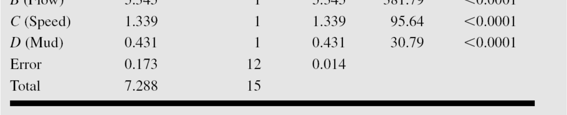
83 ANOVA for Example

84 If curvature is significant, augment the design with axial runs to create a central composite design. The CCD is a very effective design for fitting a second-order response surface model 84

85 Practical Use of Center Points (pg. 289) Use current operating conditions as the center point Check for abnormal conditions during the time the experiment was conducted Check for time trends Use center points as the first few runs when there is little or no information available about the magnitude of error Center points and qualitative factors? 85

86 Center Points and Qualitative Factors 86

87 6.9 Why We Work with Coded Design Variables P