Numerical Solution of Differential Equations

Transcription

1 Numerical Solution of Differential Equations 3 rd year JMC group project Summer Term 2004 Supervisor: Prof. Jeff Cash Saeed Amen Paul Bilokon Adam Brinley Codd Minal Fofaria Tejas Shah

2 Agenda Adam: Differential equations and numerical methods Paul: Basic methods (FE, BE, TR). Problem: circle Saeed: Advanced methods (4 th order). Problem: Kepler s equation Minal: Stiff equations Tejas: Derivation of 6 th order method

3 Agenda Adam: Differential equations and numerical methods Paul: Basic methods (FE, BE, TR). Problem: circle Saeed: Advanced methods (4 th order). Problem: Kepler s equation Minal: Stiff equations Tejas: Derivation of 6 th order method

4 Introduction to Differential Equations Equations involving a function y of x, and its derivatives Model real world systems General Equation:

5 Introduction to Differential Equations Simple example Solution obtained by integrating both sides Initial values can determine c

6 Introduction to Differential Equations Special case when equations do not involve x E.g. Initial values y(0) = 1 and y'(0) = 0, solution is

7 Introduction to Differential Equations Kepler s Equations of Planetary Motion Difficult to solve analytically we use numerical methods instead

8 Introduction to Differential Equations Forward Euler and Backward Euler Trapezium Rule General method Use initial value of y at x=0 Calculate next value (x=h for small h) using gradient Call this y 1 and repeat Need formula for y n+1 in terms of y n

9 Agenda Adam: Differential equations and numerical methods Paul: Basic methods (FE, BE, TR). Problem: circle Saeed: Advanced methods (4 th order). Problem: Kepler s equation Minal: Stiff equations Tejas: Derivation of 6 th order method

10 Agenda Adam: Differential equations and numerical methods Paul: Basic methods (FE, BE, TR). Problem: circle Saeed: Advanced methods (4 th order). Problem: Kepler s equation Minal: Stiff equations Tejas: Derivation of 6 th order method

11 Euler s Methods Simplest way of solving ODEs numerically Does not always produce reasonable solutions Forward Euler (explicit) and Backward Euler (implicit)

12 Forward Euler y True solution y(x + h) = y(x) + h y (x) Explicit y 2 Slope f(x 0, y 0 ) (x 2, y 2 ) Slope f(x 1, y 1 ) Approximated solution E loc = ½h 2 y (2) (ξ) h 2 First order Asymmetric y 1 (x 1, y 1 ) y 0 (x 0, y 0 ) h h x 0 x 1 x 2 x

13 Backward Euler y 2 y (x 2, y 2 ) y(x + h) = y(x) + h y (x + h) True solution Implicit E loc = - ½h 2 y (2) (ξ) h 2 y 1 Slope f(x 1, y 1 ) (x 1, y 1 ) Slope f(x 2, y 2 ) Approximated solution First order Asymmetric y 0 (x 0, y 0 ) h h x 0 x 1 x 2 x

14 Trapezium Rule y(x + h) = y(x) + ½ h [y (x) + y (x + h)] Average of FE and BE Implicit E loc = - (h 3 /12) f (2) (ξ) h 3 Second order Symmetric

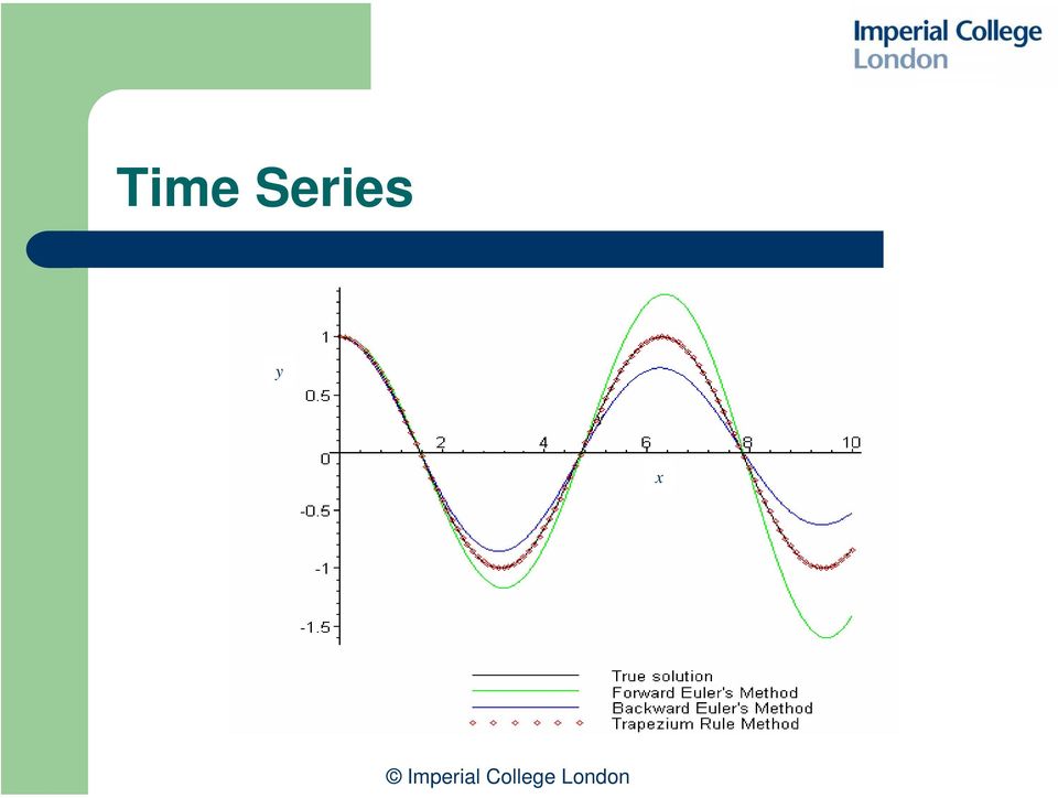
15 Example Problem: Circle Consider y = -y, with initial conditions y(0) = 1 y (0) = 0 The analytical solution is y = cos x, that can be used for comparison with numerical solutions

16 Plots for the True Solution Time series plot (xy) Phase plane plot (zy)

17 Time Series y x

18 Phase Plane Plots: FE & BE Forward Euler Backward Euler

19 Phase Plane Plots: TR FE & BE fail: non-periodic TR: OK, periodic sol n W h y?

20 Symmetricity TR is symmetric, whereas FE & BE are not Still TR! y(x + h) = y(x) + ½ h [y (x) + y (x + h)] h -h y(x - h) = y(x) - ½ h [y (x) + y (x - h)] X := x - h y(x + h) = y(x) + ½ h [y (X) + y (X + h)]

21 Symmetricity TR is symmetric, whereas FE & BE are not Still FE? y(x + h) = y(x) + h y (x) h -h y(x - h) = y(x) - h y (x) X := x - h y(x + h) = y(x) + h y (X + h)

22 Time Step h = 10-1 h = 10-2

23 Agenda Adam: Differential equations and numerical methods Paul: Basic methods (FE, BE, TR). Problem: circle Saeed: Advanced methods (4 th order). Problem: Kepler s equation Minal: Stiff equations Tejas: Derivation of 6 th order method

24 Agenda Adam: Differential equations and numerical methods Paul: Basic methods (FE, BE, TR). Problem: circle Saeed: Advanced methods (4 th order). Problem: Kepler s equation Minal: Stiff equations Tejas: Derivation of 6 th order method

25 After Euler and TR Can create higher order methods, which have far smaller global errors Methods are more complex and require more computation on each step But for same step size more accurate Introduce concept of half step

26 Two Fourth Order Methods y n+1 y n = y n + h/2(y n ) + (h 2 /12)(4y n+½ + 2y n ) y n+1 y n = h/6(y n+1 + 4y n+½ + y n ) (*) Then to calculate the half-step we use either A or B A) y n+ ½ = ½(y n+1 + y n ) h 2 /48(y n+1 + 4y n+½ + y n ) B) y n+ ½ = y n + ½y n h 2 /192(-2y n y n+½ + 14y n ) Which one is more accurate? (next slide) Solve iteratively and then apply solution to find derivative (*)

27 Creating Method A Start with y n+1 y n = h/6[y n+1 + 4y n+½ + y n ] (1) diff. y n+1 y n = h/6[y n+1 + 4y n+½ + y n ] (2) y n+½ = ½(y n+1 + y n ) h/8(y n+1 y n ) (3) diff. y n+½ = ½(y n+1 + y n ) h/8(y n+1 y n ) (4) subs (4) into (1) (to eliminate y n+½ ) and eliminate y n+1 using (2), then use (2) in (3) to get half-step

28 Comparing Fourth Order Methods Comparing errors when solving circle problem Both A and B produce a much smaller order of error than Euler s

29 Finding Earth s Orbit Around Sun Kepler s Equation Can use it to find the orbit of planets Use to find orbit of earth around the sun Work in two dimensions z and y z = -(GM z) / (y 2 + z 2 ) 3/2 y = -(GM y) / (y 2 + z 2 ) 3/2 Constants and initial conditions in report

30 Results Plot Solution uses small step size h = 0.01 Becomes difficult to tell difference between methods visually Using h = 0.1 difference is more marked

31 Agenda Adam: Differential equations and numerical methods Paul: Basic methods (FE, BE, TR). Problem: circle Saeed: Advanced methods (4 th order). Problem: Kepler s equation Minal: Stiff equations Tejas: Derivation of 6 th order method

32 Agenda Adam: Differential equations and numerical methods Paul: Basic methods (FE, BE, TR). Problem: circle Saeed: Advanced methods (4 th order). Problem: Kepler s equation Minal: Stiff equations Tejas: Derivation of 6 th order method

33 Stiff Equations Certain systems of ODEs are classified as stiff A system of ODEs is stiff if there are two or more very different scales of the independent variable on which the dependent variables are changing Some of the methods used to find numerical solutions fail to obtain the required solution

34 Example Consider the equation: 2 d y dy + ( λ + 1) + λy = 2 dx dx With initial conditions: y( 0) = y' (0) 1 = 1 There are two solutions to this problem 0

35 Example continued Analytical solution: y=e -x Unwanted solution: y=e -λx We will now show how forward Euler is not stable when solving this problem under certain circumstances

36 Example continued Let λ = 10 3 and let (the step size) h = 0.1

37 Increasing the range of the x-axis

38 When h = 0.001

39 Agenda Adam: Differential equations and numerical methods Paul: Basic methods (FE, BE, TR). Problem: circle Saeed: Advanced methods (4 th order). Problem: Kepler s equation Minal: Stiff equations Tejas: Derivation of 6 th order method

40 Agenda Adam: Differential equations and numerical methods Paul: Basic methods (FE, BE, TR). Problem: circle Saeed: Advanced methods (4 th order). Problem: Kepler s equation Minal: Stiff equations Tejas: Derivation of 6 th order method

41 A Sixth Order Numerical Method Has an error term with smallest h degree as h 7 Idea is to find values for α, A, B, C, D, E, F, C, D, E, F such that:

42 Derivation Compare Taylor s Expansion of LHS and RHS So for: First expand the LHS

43 Derivation Now expand individual terms on RHS of our expression: This gives:

44 Derivation Equate both sides and solve for constants: Similarly we can find C, D, E, F and C, D, E, F

45 Applying 6 th Order Method How to obtain results using derived method. Produce a set of simultaneous equations and solve. Find y n+1 from old values and those just obtained. Set x, y n, y n etc. to new values. Repeat above procedure with updated variables.

46 Circle Problem Example Circle is produced for phase plane plot

47 Kepler s Equations Solution obtained from z-y plot reinforces fourth order method results.

48 The End But perhaps you want more? Read our report Visit our website: