5.6 2 k p Fractional Factorial Designs

Transcription

1 5.6 2 k p Fractional Factorial Designs There are k factors of interest each having 2 levels. There are only enough resources to run 1/2 p of the full factorial 2 k design. Thus, we say we want to run a 1/2 p fraction of a 2 k design. This design is called a 2 k p fractional factorial design. Suppose there are 7 factors of interest (A, B, C, D, E, F, G). There are only enough resources for 16 experimental runs which is 1/8 of a 2 7 design. Thus, we want to run a 1/8 fraction of a 2 7 design. This design is called a fractional factorial design. When selecting a 1/2 p fraction, we want to be sure that we select design points that will enable us to estimate effects of interest. Generation of such a design (if it exists) is to carefully choose p interactions to generate the design and then decide on the sign of each generator. These p interactions are called the generators of the 2 k p fractional factorial design, and with the 2 p 1 p generalized interactions form the complete defining relation for the design. Suppose there are 7 factors and we choose ABCE, BCDF, and to be the generators of the design. Then there are 8 ways to assign signs to these: I = ±ABCE = ±BCDF = ± Each of these 8 assignments will generate a unique 1/8 fraction of a 2 7 design. Suppose we choose the (+,+,+) case: I = ABCE = BCDF =. The generalized interactions are formed by taking all 2-way and 3-way products and then reduce: ABCE BCDF = ADEF ABCE ACDG = BCDF ACDG = ABCE BCDF ACDG = Thus, the complete defining relation is given by I = ABCE = BCDF = ACDG = Because the length of the shortest word is four, this design is resolution IV, denoted a IV fractional factorial design. The 2 k p fractional factorial design is formed by selecting only those treatment combinations that have a plus signs in the p columns corresponding to the p generators. This can be accomplished in two ways: (i) List all 2 k combinations and selecting the rows with plus signs in the p columns corresponding to the p generators, OR, (ii) List all 2 k p combinations for a factorial design having k p factors. Then create columns for the remaining p factors based on the p generating interactions (i.e., the defining relation). Example: Generate the design with defining relation I = ABCE = BCDF = ACDG = ADEF = BDEG = ABF G = CEF G using method (ii). First, generate a 2 4 design in the first four factors (A, B, C, and D). Now, multiply the defining relation by E, F, and G and reduce. Choose aliases for E, F, and G in terms of A, B, C, and D only. Use these to determine the columns for E, F, and G. E = ABC = BCDEF = ACDEG = ADF = BDG = ABEF G = CF G F = ABCEF = BCD = ACDF G = ADE = BDEF G = ABG = CEG G = ABCEG = BCDGF = ACD = ADEF G = BDE = ABF = CEF 85

2 2 4 Design Treatment Look at A B C D E F G Combination ADF CF G (1) aef bef abf g cef g acf bcg abce df g adef bdeg abd cde acdg bcdf abcdef g + + Because only 1/2 p of the full factorial design is run, each of the 2 k effects (including the intercept) is aliased with 2 p 1 other effects. That is, estimation of aliased effects are calculated identically and, therefore, cannot be separated from each other. The alias structure for any 2 k p design can be determined by taking the defining relation and multiplying it by any effect. The resulting 2 p effects are all aliases. Example: In the design with defining relation I = ABCE = BCDF = ACDG = ADEF = BDEG = ABF G = CEF G, the main effects are aliased as follows: A = BCE = ABCDF = CDG = DEF = ABDEG = BF G = ACEF G B = ACE = CDF = ABCDG = ABDEF = DEG = AF G = BCEF G C = ABE = BDF = ADG = ACDEF = BCDEG = ABCF G = EF G D = ABCDE = BCF = ACG = AEF = BEG = ABDF G = CDEF G E = F = ABCEF = BCD = ACDF G = ADE = BDEF G = ABG = CEG G = ABCEG = BCDF G = ACD = ADEF G = BDE = ABF = CEF The rest of the alias structure can be generated by multiplying the defining relation by any interaction not yet appearing in a prior alias class. For example, multiply the A effect row by B, we have the alias structure for AB: AB = CE = ACDF = BCDG = = = = When determining a model for analysis, only one effect in each alias class is allowed. When estimating effects, we are actually estimating the sum of the effects in each alias class. For example, 86

3 l 1 = A + BCE + ABCDF + CDG + DEF + ABDEG + BF G + ACEF G l 2 = B + ACE + CDF + ABCDG + ABDEF + DEG + AF G + BCEF G l 3 = C + ABE + BDF + ADG + ACDEF + BCDEG + ABCF G + EF G l 4 = D + ABCDE + BCF + ACG + AEF + BEG + ABDF G + CDEF G l 5 = E + ABC + BCDEF + ACDEG + ADF + BDG + ABEF G + CF G l 6 = F + ABCEF + BCD + ACDF G + ADE + BDEF G + ABG + CEG l 7 = G + ABCEG + BCDF G + ACD + ADEF G + BDE + ABF + CEF 5.7 Minimum Aberration Designs The minimum aberration concept for two-level fractional factorial designs was introduced by Fries and Hunter (1980). When running a 2 k p fractional-factorial design, it is commonly assumed that the order of importance of effects decreases with the number of factors involved, that is, main effects are considered more important than two-factor interactions which in turn are considered more important than three-factor interactions, and so on. This is also known as the hierarchal effects principle. Given that we accept this assumption, it is desirable to choose a design of maximum resolution that is an acceptable design size. Then another practical question arises Given the set of all designs of maximum resolution, how does the experimenter select a design? By applying the minimum aberration concept this question can be answered. We say a design is a minimum aberration design if (i) it has maximum resolution and (ii) it minimizes the number or words in the defining relation of minimum length. An alternate definition of a minimum aberration design considers the alias structure. Let R max equal the maximum resolution of a 2 k p design. Then a minimum aberration design guarantees that the smallest number of main effects are confounded with interactions of order R max 1 (or equivalently, the smallest number of two-factor interactions are confounded with interactions of order R max 2, and so on). In this context, design aberration is a natural extension of design resolution. Using the notation and terminology of Chen and Lin (1991), let the elements of the defining relation be called words and the symbols comprising the words be called letters. Given a design D, let A i (D) equal the number of words of length i in the defining relation and let the vector W (D) = [A 1 (D), A 2 (D),..., A K (D)] be the wordlength or aberration pattern of D. Hence, the resolution of D equals the smallest i such that A i (D) > 0. Minimum Aberration Example 1: Consider the example presented by Fries and Hunter (1980) and by Chen and Lin (1991). In this example, we are comparing the wordlength patterns of three different designs. The generator, defining relation, and the wordlength pattern for each design are given in the following table. 87

4 Minimum Aberration Example 1 Design D 1 D 2 D 3 Generators F = ABC F = ABC F = ABCD G = BCD G = ADE G = ABCE Defining ABCF ABCF ABCDF Relation BCDG ADEG ABCEG I = Wordlength W (D 1 ) = W (D 2 ) = W (D 3 ) = Pattern As the wordlength pattern indicates, the shortest word in each defining relation is of length 4, hence, all three designs are of Resolution IV. Using aberration as a criterion to choose among the three designs, D 3 would be chosen because it has fewest words of length 4. In general, if it happened that each design had an equal number of words of minimum length R, then the number of words of length R + i where i = 1, 2,... would be compared until a design is selected. For example, suppose the wordlength patterns for three designs are (0, 0, 4, 2, 1, 0) (0, 0, 4, 1, 2, 0) (0, 0, 4, 1, 1, 1) Each design has 4 words of minimum length (length=3). Therefore, we compare the number of words of length 4. The last two designs have 1 word of length 4 and the first design has 2 words of length 4. We eliminate the first design. We now compare the number of words of length 5 for the last two designs. We select the third design because it only has 1 word of length 5 (the other design has 2 words of length 5). A minimum aberration 2 k p design is selected this way by comparing the wordlength patterns W among all 2 k p designs of maximum resolution R. Minimum Aberration Example 2: Consider the wordlength patterns of the following designs. For each design: Find the defining relation, the design resolution, and the wordlength pattern. Which design is the best based on the minimum aberration criterion? Minimum Aberration Example 2 Design D 1 D 2 D 3 D 4 Generators F = ABC F = ABC F = ABCD F = ABC G = ABD G = ABD G = BCDE G = ABDE H = BCDE H = ABCDE H = ABCDE H = ABCDE 88

5 5.8 Foldover Designs It is possible to construct resolution III designs to investigate up to N 1 factors in N runs where N is a power of 2. Let k be the number of factors of interest and let N be the smallest power of 2 such that N > k. That is, N = 2 m where m is the smallest positive integer such that 2 m > k. Use the table listing the design generators for fractional factorial designs to find the smallest 2 k p III design. More extensive tables (k > 11 factors) can be found in the experimental design literature. For example, suppose we want to study the main effects of 7 factors (A, B, C, D, E, F, G) in a resolution III design. Use the III design with generators D = ±AB, E = ±AC, F = ±BC, and G = ±ABC. The design with all pluses for its generators has the defining relation I = ABD = ACE = BCF = ABCG = = = If N 1 = k then the fractional factorial design is saturated. For a saturated design, we can estimate the k effects aliased with the k factors, but we cannot perform any hypothesis tests because there are 0 degrees of freedom for the error. Example: For k = 7 factors, the III design with generators D = AB, E = AC, F = BC, and G = ABC is saturated. Each of the 7 main effects is aliased with 15 other effects. The alias structure associated with each main effect is: A = BD = CE = ABCF = BCG = ABCDE = CDF = ACDG = BEF = ABEG = F G = ADEF = DEG = ACEF G = ABDF G = BCDEF G B = AD = ABCE = CF = ACG = CDE = ABCDF = BCDG = AEF = EG = ABF G = BDEF = ABDEG = BCEF G = DF G = ACDEF G C = ABCD = AE = BF = ABG = BDE = ADF = DG = ABCEF = BCEG = ACF G = CDEF = ACDEG = EF G = BCDF G = ABDEF G D = AB = ACDE = BCDF = ABCDG = BCE = ACF = CG = ABDEF = BDEG = ADF G = EF = AEG = CDEF G = BF G = ABCEF G E = ABDE = AC = BCEF = ABCEG = BCD = ACDEF = CDEG = ABF = BG = AEF G = DF = ADG = CF G = BDEF G = ABCDF G F = ABDF = ACEF = BC = ABCF G = BCDEF = ACD = CDF G = ABE = BEF G = AG = DE = ADEF G = CEG = BDG = ABCDEG G = ABDG = ACEG = BCF G = ABC = BCDEG = ACDF G = CD = ABEF G = BE = AF = DEF G = ADE = CEF = BDF = ABCDEF G 89

6 If we assume that 3-factor and higher interactions are negligible ( 0), then we can simplify the alias structure and the estimation structure: l A = A + BD + CE + F G l E = E + AC + BG + DF l B = B + AD + CF + EG l F = F + BC + AG + DE l C = C + AE + BF + DG l G = l D = D + AB + CG + EF Using this approach, it is possible to study up to 15 factors in a resolution III 16-run design, 31 factors in a resolution III 32-run design, etc. (but with a lot of aliasing of main effects with two-factor interactions). We can increase the number of main effects that can be isolated and estimated independently of other two-factor interactions by applying a sign-changing procedure. In this procedure we take a resolution III fractional factorial design and add a second fraction that is formed by changing the signs of all of the levels in the k main effect columns. This is called folding over the design. The design formed by combining the two-fractions is called a foldover design and will allow estimation of all main effects independently of any 2-factor interaction. Example: Suppose we fold over the design having the defining relation in (7). We would then get the following foldover design. You must examine the D, E, F and G columns to attach the correct sign to an alisased interaction. Included are sample data for analysis. First Half of Foldover Design A B C D = E = F = G = Sample AB AC BC Data Second Half of Foldover Design A B C D = E = F = G = Sample Data

7 This second folded-over fraction has defining relation: I = ABD = ACE = BCF = ABCG = BCDE = ACDF = CDG = ABEF = BEG = AF G = DEF = ADEG = CEF G = BDF G = ABCDEF G. Note that the sign for any interaction involving an even number of effects did not change while the sign for any interaction involving an odd number of effects did change. The alias structure associated with each main effect in the folded-over fraction is: A = BD = CE = ABCF = BCG = ABCDE = CDF = ACDG = BEF = ABEG = F G = ADEF = DEG = ACEF G = ABDF G = BCDEF G B = AD = ABCE = CF = ACG = CDE = ABCDF = BCDG = AEF = EG = ABF G = BDEF = ABDEG = BCEF G = DF G = ACDEF G C = ABCD = AE = BF = ABG = BDE = ADF = DG = ABCEF = BCEG = ACF G = CDEF = ACDEG = EF G = BCDF G = ABDEF G D = AB = ACDE = BCDF = ABCDG = BCE = ACF = CG = ABDEF = BDEG = ADF G = EF = AEG = CDEF G = BF G = ABCEF G E = ABDE = AC = BCEF = ABCEG = BCD = ACDEF = CDEG = ABF = BG = AEF G = DF = ADG = CF G = BDEF G = ABCDF G F = ABDF = ACEF = BC = ABCF G = BCDEF = ACD = CDF G = ABE = BEF G = AG = DE = ADEF G = CEG = BDG = ABCDEG G = ABDG = ACEG = BCF G = ABC = BCDEG = ACDF G = CD = ABEF G = BE = AF = DEF G = ADE = CEF = BDF = ABCDEF If we assume that 3-factor and higher interactions are negligible ( 0), then we can simplify the alias structure and the estimation structure of the second fraction: l A = A BD CE F G l B = B AD CF EG l C = C AE BF DG l D = D AB CG EF l E = E AC BG DF l F = F BC AG DE l G = G CD BE AF Main effect estimates for A: First half: A + A = = Second half: A + A = = Why are the estimates of the A main effect so different between the two halves of the foldover design? The reason is the alias structure. 91

8 From the first half of the design we get: l A = A + BD + CE + F G l E = E + AC + BG + DF l B = B + AD + CF + EG l F = F + BC + AG + DE l C = C + AE + BF + DG l G = G + CD + BE + AF l D = D + AB + CG + EF From the second half of the design we get: l A = A BD CE F G l E = E AC BG DF l B = B AD CF EG l F = F BC AG DE l C = C AE BF DG l G = G CD BE AF l D = D AB CG EF Assume that 3-factor and higher interactions are negligible. If we take the two linear combinations (l i + l i)/2 and (l i l i)/2, we get i (l i + l i)/2 (l i l i)/2 A A = 1.48 BD + CE + F G = B B = AD + CF + EG = 0.33 C C = 1.80 AE + BF + DG = 1.53 D D = AB + CG + EF = 0.50 E E = 0.13 AC + BG + DF = 0.40 F F = 0.50 BC + AG + DE = 1.53 G G = 0.13 CD + BE + AF = 2.55 Note that we have isolated all of the main effects from every 2-factor interaction. The two largest effects are B and D. Because the third largest effect is the BD + CE + F G, it seems reasonable to attribute this to the BD interaction. Note: Because the two halves of the foldover design are run sequentially, a blocking variable should be included in the model. We also use the same tools for analyzing data from an unreplicated 2 k design: study a normal probability plot of estimated effects and then pool terms with small estimated effects to form the MSE SAS Code and Output for the Foldover Design Example **************************************; *** THE FIRST HALF OF THE FOLDOVER ***; **************************************; DATA IN; DO C = -1 TO 1 BY 2; DO B = -1 TO 1 BY 2; DO A = -1 TO 1 BY 2; D = A*B; E=A*C; F=B*C; G=A*B*C; INPUT OUTPUT; END; END; END; CARDS; PROC GLM DATA=IN; CLASS A B C D E F G; MODEL Y = A B C D E F G / SS3; ESTIMATE A A -1 1; ESTIMATE B B -1 1; ESTIMATE C C -1 1; ESTIMATE D D -1 1; ESTIMATE E E -1 1; ESTIMATE F F -1 1; ESTIMATE G G -1 1; TITLE THE FIRST HALF OF THE FOLDOVER ; 92

9 ***************************************; *** THE SECOND HALF OF THE FOLDOVER ***; ***************************************; DATA IN2; DO C = 1 TO -1 BY -2; DO B = 1 TO -1 BY -2; DO A = 1 TO -1 BY -2; D = -A*B; E=-A*C; F=-B*C; G=A*B*C; INPUT OUTPUT; END; END; END; CARDS; PROC GLM DATA=IN2; CLASS A B C D E F G; MODEL Y = A B C D E F G / SS3; ESTIMATE A A -1 1; ESTIMATE B B -1 1; ESTIMATE C C -1 1; ESTIMATE D D -1 1; ESTIMATE E E -1 1; ESTIMATE F F -1 1; ESTIMATE G G -1 1; TITLE THE SECOND HALF OF THE FOLDOVER ; *****************************************; *** THE FULL FOLDOVER DESIGN ANALYSIS ***; *****************************************; DATA IN; SET IN; BLOCK=1; DATA IN2; SET IN2; BLOCK=2; DATA BOTH; SET IN IN2; PROC GLM DATA=BOTH; CLASS A B C D E F G BLOCK; MODEL Y = BLOCK A B C D E F G B*D A*D A*E A*B A*C B*C C*D / SS3; ESTIMATE A A -1 1; ESTIMATE B B -1 1; ESTIMATE C C -1 1; ESTIMATE D D -1 1; ESTIMATE E E -1 1; ESTIMATE F F -1 1; ESTIMATE G G -1 1; ESTIMATE B*D B*D / DIVISOR=2; ESTIMATE A*D A*D / DIVISOR=2; ESTIMATE A*E A*E / DIVISOR=2; ESTIMATE A*B A*B / DIVISOR=2; ESTIMATE A*C A*C / DIVISOR=2; ESTIMATE B*C B*C / DIVISOR=2; ESTIMATE C*D C*D / DIVISOR=2; TITLE BOTH HALVES OF THE FOLDOVER DESIGN ; RUN; 93

10 SAS Output: THE FIRST HALF OF THE FOLDOVER Dependent Variable: Y Sum of Mean Source DF Squares Square F Value Pr > F Model Error 0.. Corrected Total Source DF Type III SS Mean Square F Value Pr > F A B C D E F G T for H0: Pr > T Std Error of Parameter Estimate Parameter=0 Estimate A B C D E F G ======================================================================= THE SECOND HALF OF THE FOLDOVER Dependent Variable: Y Sum of Mean Source DF Squares Square F Value Pr > F Model Error 0.. Corrected Total Source DF Type III SS Mean Square F Value Pr > F A B C D E F G T for H0: Pr > T Std Error of Parameter Estimate Parameter=0 Estimate A B C D E F G

11 BOTH HALVES OF THE FOLDOVER DESIGN Dependent Variable: Y Sum of Mean Source DF Squares Square F Value Pr > F Model Error 0.. Corrected Total Source DF Type III SS Mean Square F Value Pr > F BLOCK A B C D E F G B*D A*D <-- Pool A*E A*B <-- Pool A*C <-- Pool B*C C*D T for H0: Pr > T Std Error of Parameter Estimate Parameter=0 Estimate A B C D E F G B*D A*D A*E A*B A*C B*C C*D

12 5.9 Plackett-Burman Designs Plackett and Burman (1946) designs are two-level fractional factorial designs for studying a maximum of k = N 1 factors in N experimental runs where N is a multiple of 4. If N is a power of 2, then these designs are the resolution III fractional factorial designs. We will examine the case when N is a multiple of 4 but not a power of 2 (such as, N = 12, 20, 24, 28, 36). These designs are generated as follows: 1. Form the first column from the generating sequence of N/2 pluses and N/2 1 minuses. N = 12 N = N = N = The second column is generated from the first column by moving the elements in the first column down one position and placing the last element in the first position. 3. The remaining columns are constructed similarly from the previous column. 4. After the N 1 rows and columns are generated, add a row of minus signs to complete the design. Example: Generate the 12-point Plackett-Burman design. Step 1: Enter the vector of + and signs in the factor A column. Plackett-Burman design for N = 12 Run A B C D E F G H I J K Step 2: Fill in the factor B column by shifting the factor A column down 1 row. The last sign is put in the first row of factor B. Plackett-Burman design for N = 12 Run A B C D E F G H I J K

13 Step 3: Fill in columns C to K using the procedure in Step 2; Plackett-Burman design for N = 12 Run A B C D E F G H I J K Step 4: Fill in last row with signs. Plackett-Burman design for N = 12 Run A B C D E F G H I J K In practice, we randomly assign the k factors to k of the columns in the Plackett-Burman design and then randomize the run order. Each unassigned column corresponds to one degree of freedom for error. It is recommended that at least 4 columns be left unassigned for error estimation. Plackett-Burman designs for N = 12, 20, 24, 28, and 36 have very complicated alias structures. For example, in the 12-run design, each main effect is partially aliased with the 45 two-factor interactions that do not involve itself. 97

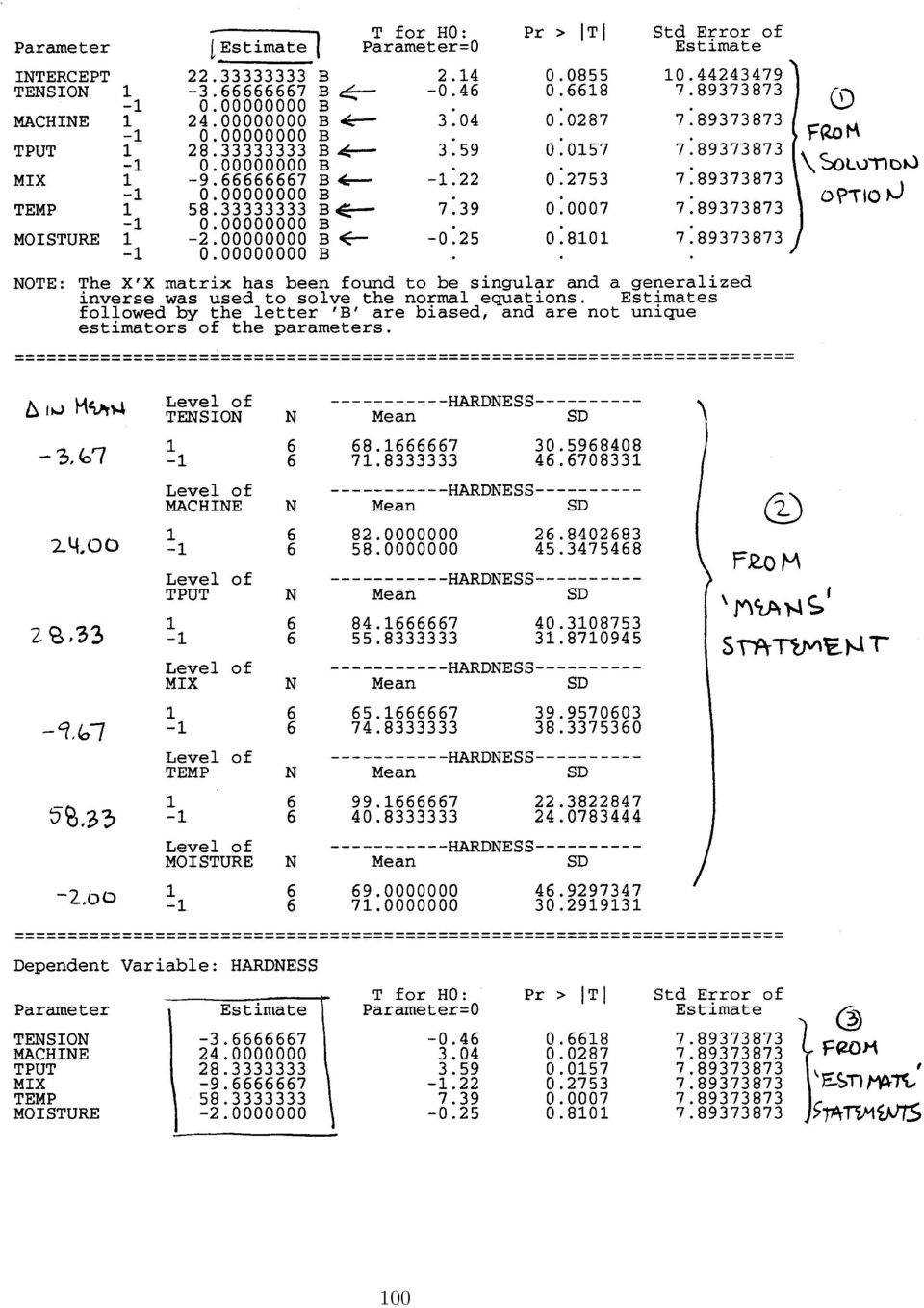
14 5.9.1 Plackett-Burman Design Example A 6-factor 12-run Plackett-Burman design was run. The factors of interest were (1) tension control, (2) machine, (3) throughput, (4) mixing procedure, (5) temperature, and (6) moisture level. 98

15 Plackett-Burman Design Example DATA IN; INPUT TENSION MACHINE TPUT MIX TEMP MOISTURE HARDNESS CARDS; ; PROC GLM DATA=IN; CLASS TENSION MACHINE TPUT MIX TEMP MOISTURE ; (1) MODEL HARDNESS = TENSION MACHINE TPUT MIX TEMP MOISTURE / SOLUTION SS3; MEANS TENSION MACHINE TPUT MIX TEMP MOISTURE ; (2) ESTIMATE TENSION TENSION -1 1; --+ ESTIMATE MACHINE MACHINE -1 1; ESTIMATE TPUT TPUT -1 1; (3) ESTIMATE MIX MIX -1 1; ESTIMATE TEMP TEMP -1 1; ESTIMATE MOISTURE MOISTURE -1 1; --+ TITLE ANOVA FOR PLACKETT-BURMAN EXAMPLE ; RUN; ======================================================================= ANOVA FOR PLACKETT-BURMAN EXAMPLE General Linear Models Procedure Dependent Variable: HARDNESS Sum of Mean Source DF Squares Square F Value Pr > F Model Error Corrected Total R-Square C.V. Root MSE HARDNESS Mean Source DF Type III SS Mean Square F Value Pr > F TENSION MACHINE <-- TPUT <-- MIX TEMP <-- MOISTURE

16 100