Crosstalk Coupling: Single-Ended vs. Differential

Transcription

1 TECHNICAL PUBLICATION Crosstalk Coupling: Single-Ended vs. Differential Douglas Brooks, President UltraCAD Design, Inc. September

2 ABSTRACT The paper begins with four propositions. 1), the effects of crosstalk coupling decrease with trace separation. 2), crosstalk coupled to a differential pair has meaning only for the differential component of the crosstalk on the differential pair, not the common mode component of the crosstalk. A differential component only exists because the outside trace is (perhaps only slightly) further away from the source than is the inside trace. 3), crosstalk caused by a differential pair would be equal and opposite, and therefore cancel, on a victim trace were it not for the (perhaps only slight) separation of the differential traces themselves. Since one trace (of the pair) is (slightly) closer to the victim trace than is the other trace of the differential pair, that trace will couple slightly more strongly and there will be a small differential coupling to a victim trace. 4), differential pair coupling to another differential pair would combine these last two effects and should be quite small. The relationships between these four propositions are quantified and then tested against four PCB structures using the Mentor Graphics Hyperlynx simulation tool. The four structures are: microstrip, deeply embedded microstrip (with a thick dielectric layer above the trace), balanced stripline, and asymmetric stripline. The results of the simulations are as predicted for microstrip configurations and for stripline configurations when the traces are close together relative to the second reference plane. But singleended coupling drops off more quickly than predicted with increased spacing for stripline environments. Differential coupling, however, does not drop off in the same manner for stripline configurations. INTRODUCTION AND BACKGROUND Crosstalk is often a serious consideration in PCB design. It is reasonably well understood that the primary strategies available to board designers for reducing crosstalk between traces are (a) rout sensitive traces close to their underlying reference planes and (b) spread the traces apart 1. How "close" and how "far" are policy variables, the responsibilities for which are usually reserved for the circuit or system design engineer. A benefit often ascribed to the use of differential signals and traces is that they are less susceptible to radiated noise (and therefore crosstalk), and that they radiate less noise (and therefore cause less crosstalk) than ordinary single-ended traces 2. If this benefit is true (and it is) then the worst PCB crosstalk environment (all other things equal) would be where a single-ended aggressor trace couples into a singleended victim trace, and the best environment would be where a differential aggressor pair couple into a differential victim pair. The case of a differential aggressor pair coupling into a single-ended victim, or of a single ended aggressor trace coupling into a differential victim pair would represent environments somewhere between the other two extremes. Typically, after board stackup decisions are made, the only variable left to control crosstalk is the spacing between traces. Thus, system engineers may give board designers layout rules for spacing. A typical rule may be spacing between traces of 5*H (H being the height above the plane, for example). These types of rules may be derived through simulations, or they may simply be "carry-overs" from previous designs, previous engineers, or even previous companies! When (and if) these layout rules are supplied, they are usually done so without regard to the types of signals (single-ended or differential) being routed. But if the degree of crosstalk is a function of the types of signals being routed, then the layout rules should (presumably) reflect this. The purpose of this paper is to look at the various signal and trace environments and compare them from a crosstalk standpoint. Given a better quantitative understanding of the relative magnitude of the crosstalk noise signals for these different environments, it may be possible to adjust layout rules more intelligently for more efficient use of board real estate. COUPLING THEORY Figure 1 illustrates typical traces that might exist on a Figure 1: Typical traces on a PCB. PAGE 1

3 PCB. These may all be single-ended traces, or either pair of traces, a and b for example, or alternatively c and d, may form a differential pair. Howard Johnson states that the coupled noise between any two traces on a PCB is proportional to 3 : Equation 1 where S is the centerline spacing between the traces (as shown in Figure 1) and H is the height of the trace above the underlying plane. Note that trace width does not enter this equation. That is not because trace width does not have an effect, it is because the width is a second-order effect, much smaller than the other variables. This proportionality can be converted into an equality by simply adding a proportionality constant, k, to the equation: Equation 2 The proportionality constant, k, covers such things as structure (stripline or microstrip for example), rise time, coupled length, etc. Presumably, k will be a constant for all of the analyses below, since the environment is "all other things equal." Thus for individual analyses we will normalize the results by assuming k = 1. For relative analyses, k will cancel out (since it appears in both the numerator and the denominator.) Finally, we are going to make one simplifying assumption here to simplify the algebra. We will assume that the ratio S/H = 1.0, that is, that the normalized spacing between the traces is equal to the height of the trace above the plane. It turns out that this has very little consequence in our theoretical discussion. We will express trace separation in terms of units of n; that is, where trace separation = n*(s/h). Thus, this has no real effect on the results of our analyses, but it greatly simplifies the algebra. Therefore, the coupled noise from Trace a on Trace b is simply: Equation 3 The coupled noise from Trace a on Trace c is: Equation 4 And, finally, the coupled noise from Trace a on Trace d is: Equation 5 The next four sections of the paper will specifically develop the theoretical concepts for the coupling of the four cases suggested in the introduction. Case A - Single ended coupling between Trace b and Trace c. The noise on Trace c from a signal on Trace b is given by: Equation 6 Presumably this is the worst-case coupling environment. As expected, the coupled noise decreases as n increases; that is, the noise decreases as the traces spread further apart. This equation will be the baseline equation for subsequent analyses. Letting k be 1.0 gives us Figure 2 for a curve of the normalized noise as a function of n: Figure 2: The normalized coupled noise on Trace c caused by a signal on Trace b as a function of n. PAGE 2

4 Case B - Single ended coupling to differential pair Trace c and Trace d. Now let Trace c and Trace d form a differential pair. A signal on Trace b will couple into each trace. In the case of a differential pair, we are only concerned with the differential noise component, not the common mode component. At first glance, we might assume that the coupled noise will be equal on both Trace c and Trace d and will therefore cancel out. Indeed, if Trace c is far enough away from Trace b this is not an unreasonable assumption. But Trace d is one unit further away from Trace b than is Trace c, so the coupled noise on Trace d will be slightly smaller than will be the coupled noise on Trace c. Therefore, there will be a small differential component of the coupled noise on the differential pair Noise on c is given, as above, by: Equation 6 Noise on d is given by: Equation 7 The common mode noise on c and d cancels out at the input, so the relevant noise is the difference between these two noise figures: Differential mode noise is Note that in Equation 10 the (k/k) term exactly cancels out. The k terms are the same (we assume) because the traces are in the same environment. This ratio (Equation 10) gets very large as n increases, meaning that the differential mode noise is very small compared to the single-ended noise. In the limit, as n increases, the noise components are nearly equal on both victim traces, and the differential noise component (Equation 8) approaches zero. When n=1 the single-ended noise (under these assumptions) is.5. When n approaches zero, the single-ended noise approaches 1.0 (perfect coupling). Therefore, as n approaches zero, the differential noise is the difference between these two single-ended conditions, or.5. So as n gets very small, the ratio between the single-ended and differential noise approaches 1/.5, or 2.0. Thus, as n approaches its alternative limits, these results are as one would expect. The figures below illustrate the normalized coupled noise from Trace b to the differential pair (Trace c and Trace d) Equation 8, and the ratio of the single-ended coupled noise to the differential coupled noise, Equation 10. Figure 4 shows that there is an improvement in coupled noise reduction offered by the differential mode case, compared to the single-ended case, ranging from a factor of about 2 to 6 as n (related to the distance between the traces) increases from about 2 to 10. Equation 8 It is expected that the single-ended noise will be much higher than the differential mode noise. The ratio of the single-ended noise (SEnoise), Case A, to the differential-mode noise (DMnoise), Case B, equals: Equation 9 or, more simply: Equation 10 Figure 3: The normalized coupled noise on the differential pair, Trace c and Trace d, caused by a signal on Trace b as a function of n (from Eq. 8). PAGE 3

5 noise, we can form the ratio as follows: Equation 14 This can be simplified slightly as follows: Equation 15 Figure 4: The ratio of the coupled noise from a single-ended driver (Trace b) on a single-ended Trace c compared to a differential pair Trace c and Trace d (from Eq. 10). Case C - Differential pair coupling to single-ended Trace C This time, let Trace a and Trace b be a differential pair, so that the signals on them are equal and opposite. As before, the noise coupled from trace b to trace c is Equation 11 It can be shown that the noise signal coupled from Trace a to Trace c is: Equation 12 When we compare Equation 8 and Equation 13, we see that they are exactly the same. And, when we compare Equation 9 and Equation 15 we see that they are the same also. Thus, the two environments, a single-ended trace coupling into a differential pair (Case B), or a differential pair coupling into a singleended trace (Case C), behave exactly the same from a crosstalk standpoint. Case D - Differential Pair coupling to differential pair Trace c and Trace d. Let Trace a and Trace b be a differential pair, so that the signals on them are equal and opposite. As before, the noise coupled from Trace b to Traces c and d, respectively, is Equation 6 Equation 7 Note that the noise signals from Trace a are opposite in sign from those from Trace b. Thus, the total coupled noise on Trace c from Trace a and Trace b is Equation 13 It can be shown that the noise signals coupled from Trace a to Traces c and d are: Equation 12 Note that this figure approaches zero as n gets very large. If n approaches zero, this figure approaches -.5. Thus, differential traces coupling into a single-ended trace create a smaller coupled signal than does a single-ended trace coupling into the same singleended trace, all other things equal. Again, this is as we would expect. And if we want to consider the ratio of the single ended coupled noise to the differential mode radiated Equation 16 Note that the noise signals from Trace a are opposite in sign from those from Trace b. Thus, the total coupled noise on Trace c from Trace a and Trace b is PAGE 4

6 Equation 13 And the total coupled noise on Trace d from Trace a and Trace b is Equation 17 Finally, since we are concerned only with the differential mode component of this noise, we are interested in The figures below illustrate the normalized coupled noise from the differential pair (Trace a and Trace b) to the differential pair (Trace c and Trace d), Equation 19 (Figure 5), and the ratio of the single-ended coupled noise to the differential coupled noise, Equation 21 (Figure 6). Figure 6 shows that there is an improvement in coupled noise reduction offered by the differential pair case (Case D), compared to the singleended case (Case A), ranging from a factor of about 4 to 25 as n (related to the distance between the traces) increases from about 2 to 10. Equation 18 Which becomes Equation 19 Note that this figure approaches zero as n gets very large. If n approaches zero, this figure approaches.20. Thus, differential traces coupling into another differential pair creates a smaller coupled signal than a single-ended trace coupling into the same differential pair, all other things equal. Again, this is as we would expect. Figure 5: The normalized coupled noise on the differential pair, Trace c and Trace d, caused by a differential signal on Trace a and Trace b as a function of n (from Eq. 19). Finally, if we want to consider the ratio of the single ended coupled noise to the differential mode radiated noise, we can form the ungainly ratio as follows: Equation 20 This can be simplified slightly as follows: Equation 21 Figure 6: The ratio of the coupled noise from a single-ended driver (Trace b) on a single-ended Trace c compared to the noise from a differential pair Trace a and Trace b on another differential pair, Trace c and Trace d (from Eq. 21). As before, the "k" term drops out. PAGE 5

7 SUMMARY The results of these cases are summarized in Table 1. N is a normalized variable representing spacing between traces or sets of traces. Recall we started with the proportional relationship for crosstalk coupling shown in Equation 1 and made the simplifying assumption that S (the centerline separation between traces) would equal H (the height of the trace above the reference plane.) Trace separation, then, is equal to n*s. Cases A through D are as described above. Recall that Case B and Case C are symmetrical and have identical results. The columns labeled "Case" in the table represent the normalized coupling coefficients for the three cases. They have little absolute meaning, but they have very real meaning as functions of the variable n and in relationship to each other. The column labeled "Ratio" is the ratio of the Case A "Case" to each of the other cases. The column labeled "1/Ratio" is simply the inverse of the Ratio column. SIMULATIONS A detailed discussion of the simulation models used in the analysis is included in Appendix 1 and the raw data recorded from those simulations is included in Appendix 2. This section of the paper will summarize the highlights of the analysis. Four structures were modeled: microstrip, "deeply" embedded microstrip, balanced stripline, and asymmetric stripline. The deeply embedded microstrip actually simulated microstrip traces in a homogeneous environment (with dielectric above and below the trace). Case A - Single ended coupling between Trace b and Trace c. If the proportionality constant, k, is a constant for all cases in all models, then the results should follow the form of Case A shown in Table 1. Note that a control measure of Case A was recorded in every simulation. The detailed results are included in Appendix 2. For the most part, the Case A results for each simulated structure are very close to each other (as we would expect). These have been averaged and are summarized in Table 2. Table 1 - Summary of the results from the various case analyses. We can interpret the results as follows. Assume we have a layout where n = 5. There would be a certain amount of crosstalk coupling between two singleended traces so described. If one of the single-ended traces were a differential pair (either the driving/aggressor trace or the victim trace) the crosstalk coupling would be lower by a factor of 3.4. If both traces were differential pairs, the crosstalk coupling would be lower by a factor of 8.7. For two single-ended traces the normalized crosstalk coupling at n=7 is.02. If one trace is a differential pair, we can achieve the same degree of crosstalk with an approximate trace separation of n = 4. If both traces are differential pairs, we can achieve the same degree of coupling with a separation of n = 3. These results, then, may offer some guidelines and comparisons for achieving satisfactory crosstalk performance on boards while at the same time reducing board routing area. Table 2 - Case A results averaged for each structure. For closely spaced traces, the results suggest the coupling is slightly stronger for stripline configurations than for microstrip configurations. This tendency is not very strong and could simply be the result of approximations that are inherent in the modeling. As the separation between traces increases the reverse tends to be true, microstrip traces couple more strongly than do stripline traces. This effect is real and is explained by the fact that as traces move further apart, the influence of the two planes becomes more important. The absolute results shown in Table 2 may not be as meaningful as the pattern between individual PAGE 6

8 analyses. Table 3 presents the same results in a different manner. The value recorded for each individual trace separation is normalized to the value for the closest separation. The normalized value for Case A from Table 1 is included in Table 3 for comparison. Table 3 - Table 2 results normalized. It is interesting that the (deeply) embedded microstrip result follows the theoretically expected pattern almost exactly. This suggests that the theory may work best for (a) microstrip traces (b) in uniform environments. The standard microstrip structure provides results that are almost as close. But the stripline results diverge as spacing increases. That is, stripline coupling decreases more than the theory would predict as trace separation increases. This effect is significantly more pronounced for the balanced stripline case than it is for the unbalanced case (which more closely resembles the deeply embedded microstrip case.) Figure 7 illustrates the Field Solver results for the embedded microstrip and the balanced stripline simulations for Case A with 36 mils (n=5) spacing. One can visualize how the presence of the upper plane attracts the electric field lines and pulls them from the victim trace, reducing the coupling to the victim. Figures 7a and b - Field solver results for 36 mil separation for the embedded microstrip (a, below - left) and for the balanced stripline (b, above) Case A simulations. Case B - Single ended coupling to differential pair Trace c and Trace d. Table 4 illustrates the specific results for Case B (a single-ended trace coupling to a differential pair) for the microstrip simulation. The Case A column records the specific single-ended coupling results recorded for this simulation. Case B Trace c and Trace d columns, respectively, record the data for the coupling of this trace to the differential pair. Note that, in theory, the Case B/Trace c data should equal the Case A/Trace b data for each row. It is conceptually the same coupling. Similarly, the Case B/Trace d data (for any row, n) should (conceptually) be the same as the Case A/Trace b data for the next row (n+1). The data show that this is approximately true, but not exactly. This probably simply reflects the limits of this type of modeling investigation. Table 4 - Case B results for microstrip. PAGE 7

9 Table 4 also records the calculated Case B ratio (for microstrip) and compares that to the reference data (from Table 1). The overall fit is quite good. The specific results for the other three configurations can be found in Appendix 2. Table 5 summarizes the calculated ratios for the four configurations. Recall that the ratio is the single-ended case (a single ended trace coupling into another single-ended trace) divided by the case under study (in this case a single-ended trace coupling into a differential pair). For closely spaced traces, this ratio behaves approximately as predicted. And, for both microstrip configurations, this ratio also behaves approximately as predicted. But for the stripline configurations the ratio plateaus fairly quickly and stops increasing. Figure 8 - Representative field solver pattern for Case B, balanced stripline. Case C - Differential pair coupling to single-ended Trace C The Case C results roughly correspond to the Case B results, as shown in Table 6. The same discussions and the same conclusions apply to Case C as apply to Case B. Table 5 - Case B results as a function of structure. Thus, for example, the single-ended to single ended coupling at a spacing of n=8 is approximately 4.5 times stronger than the single-ended to differential pair coupling at the same separation for microstrip configurations, but only about 1.6 to 2.2 times stronger for stripline configurations. The stripline results reflect a combination of two effects that are interacting. The first is that in stripline all coupling decreases more sharply with distance because of the added influence of the second reference plane. But also in stripline, there is an inherent shielding that is going on. The inside trace of the differential pair is tending to shield the coupling to the outside trace. This is suggested by the field solver picture shown as Figure 8. Thus, the differential component of the coupled noise tends to be stronger because most of the coupling is to the inner trace. Table 6 - Case C results as a function of structure. Case D - Differential Pair coupling to differential pair Trace c and Trace d. Finally, the Case D results also mirror the previous discussions. The summary results are shown in Table 7. Table 7 - Case D results as a function of structure. PAGE 8

10 The microstrip and embedded microstrip simulation results are reasonably consistent with the theory. The stripline results, however, tend to plateau fairly quickly. The balanced stripline simulation plateaus more quickly then does the asymmetric stripline simulation because the second plane exerts its influence at closer separations. The asymmetric stripline results plateau at a slightly higher level than the balanced stripline case. This is primarily the result of the fact that there is stronger coupling between all traces in the unbalanced stripline case than in the balanced stripline case. That is, the influence of the upper plane is less because it is further away. Consequently, there is more coupling to the outer trace (Trace d) of the differential pair in the asymmetric stripline case, and therefore (relatively speaking) a stronger common-mode component of the coupling that is cancelled out at the receiver. A field solver pattern for Case D is shown in Figure 9. mode component of the crosstalk. A differential component only exists because the outside trace is (perhaps only slightly) further away from the source than is the inside trace. Third, crosstalk caused by a differential pair would be equal and opposite, and therefore cancel, on a victim trace were it not for the (perhaps only slight) separation of the differential traces themselves. Since one trace (of the pair) is (slightly) closer to the victim trace than is the other trace of the differential pair, that trace will couple slightly more strongly. Fourth, crosstalk caused by a differential pair coupling to another differential pair will result in, relatively speaking, a very small differential crosstalk signal. Equation 1 does not predict an absolute value of coupling; it only provides a proportional relationship. Thus, the theoretical results are not particularly meaningful in themselves, except as they relate to each other. It is the relationship that can be evaluated and tested. Table 1 summarizes the expected relationships for the four types of coupling scenarios. Several Hyperlynx models were developed and evaluated. Four structures were modeled --- microstrip, deeply embedded microstrip, balanced stripline, and asymmetric stripline. The four coupling scenarios were modeled for each of the four structures and their results compared to the expected results shown in Table 1. Figure 9 - Representative field solver pattern for Case D, asymmetric stripline. SUMMARY AND CONCLUSIONS This paper began with some hypothetical traces (Figure 1) and a crosstalk coupling relationship (Equation 1.) Several different trace coupling scenarios were developed and their theoretical results compared. First, the effects of crosstalk coupling are expected to decrease with trace separation proportional to Equation 1. Second, crosstalk coupled to a differential pair has meaning only for the differential component of the crosstalk on the differential pair, not the common The results for the simulation models of the microstrip and deeply embedded microstrip structures were roughly as predicted from Table 1 for all four coupling scenarios. The results for the simulations of the balanced and asymmetric stripline structures were roughly as predicted for closely spaced traces. But as the trace separation increased the results deviated from those predicted. The degree of deviation was greater for the balanced stripline case than for the asymmetric stripline case. The reason for the deviation is two-fold. First, crosstalk coupling falls off much more quickly with separation once the influence of the second reference plane is felt. This happens at closer spacing for the balanced stripline than it does for the asymmetric stripline structures. PAGE 9

11 Then, the differential component of the crosstalk coupling is relatively stronger for the stripline cases than is predicted because (a) the crosstalk coupling falls off more quickly because of the increased distance to the "outside" traces of the differential pair, and (b) there is an effective "shielding" of the outside traces that begins to have an effect. Thus, most of the coupling with differential traces in stripline environments is differential coupling rather than common mode coupling (i.e. equal on both traces.) IMPACT ON TRACE ROUTING GUIDELINES We often express PCB crosstalk design guidelines as some multiple of H (where H is the height of the trace above the reference plane.) For example, we might say we want traces spaced 5H apart. Looking at Table 3, consider a single-ended spacing represented by n=8. The simulation suggests we can meet that crosstalk target with an "n" equal to 7 or 8 for microstrip, but with an "n" of only 5.5 to 7.5 for stripline. Thus, stripline gives us a slight advantage over microstrip, and this advantage increases sharply as n increases. environments (especially balanced stripline) than it does in microstrip environments. Thus board geometry can possibly be reduced by placing single-ended crosstalk-sensitive traces in stripline environments. On the other hand, with differential traces there is only marginal benefit from placing differential pairs on stripline layers compared to microstrip layers. FOOTNOTES. 1. It has also been shown that terminations sometimes have an effect on crosstalk. See, for example, Brooks, Douglas, Signal Integrity Issues and Printed Circuit Board Design, Prentice Hall, 2003, p. 229 and especially p Ibid. p Johnson, Howard and Graham, Martin; High-Speed Digital Design, A Handbook of Black Magic, Prentice Hall, 1993, p Differential coupling is predicted to be much smaller than single-ended coupling because a large part of the coupling is canceled (differential aggressors) or common mode (differential victims). When we have both differential aggressors and differential victims these effects combine to greatly reduce coupling compared to the same spacing for single-ended traces. The simulation models confirm these expected results for microstrip configurations. For separations equivalent to n=8 the microstrip coupling is approximately 4.5 times those for Case B and Case C and approximately 15 times that for Case D. But for stripline these coupling ratios are not manifested. The n=8 couplings are only about 2.2 to 2.6 times those for Case B and Case C for asymmetric stripline and only about 1.6 to 2.0 for balanced stripline. The Case D coupling ratio is only about 6 times for asymmetric stripline and about 3 times for balanced stripline. Most of this reduced coupling ratio is caused by the fact that single-ended coupling falls off more quickly in stripline environments. BOTTOM LINE: If we are concerned about crosstalk coupling between single ended traces, the coupling reduces much more quickly with increased separation in stripline PAGE 10

12 APPENDIX 1 - SIMULATION MODELS Four structures were modeled in this analysis: microstrip, deeply embedded microstrip, balanced (or centered) stripline, and unbalanced (or asymmetric) stripline. These stackups are summarized in Figure A1a and Figure A1b, below. where H1 is the height to the upper plane and H2 is the height to the lower plane. For balanced stripline, H1 and H2 must equal 16 to achieve an "equivalent" H of 8. In an asymmetric structure, there is no unique combination of H1 and H2 that equals 8; there are an infinite number of combinations that can achieve that result. For this investigation, I selected an H1 = 40 and H2 = 10 for the asymmetric case as a reasonable set of values. These are illustrated in Figure A1a and Figure A1b. Figure A1a - Typical stackup model for microstrip and balanced stripline. Figure A1b - Typical stackup for deeply embedded microstrip and unbalanced stripline. The microstrip and deeply embedded microstrip trace layers are placed 8 mils above the underlying plane. This represents the value for the variable "H" in Equation 1. If we want to be able to compare the results of the stripline models to the microstrip models, then the effective (or equivalent) H must also be 8 mils in those stackups. I have shown in previous papers A1 that the equivalent H in stripline models is the parallel combination of the heights to each of the reference planes. That is: Heq = H1*H2/(H1+H2) Figure A2 - Typical trace layer organization. Figure A2 illustrates a typical trace layer. In all analyses, the trace layers are organized as a variation of this orientation. There are two sets of traces, as shown. These traces always correspond to Traces a, b, c, and d as shown in Figure 1 of the paper. Consider the pair on the left. This pair either represents a differential pair (if they are coupled in the model) or the inner (right-hand) trace (only) is used as a single, single-ended trace. The right-hand pair also represents a differential pair (if they are coupled in the model) or else the inner (left-hand) trace is used as a single, single-ended trace. The traces are all modeled as 4 mils wide and 36 inches long, and their impedance is calculated by the Hyperlynx tool depending on the specific structure, configuration and orientation. Figure A2 specifically represents the case of a basic microstrip structure with two differential pairs. Note how this orientation is representative of Figure 1 in the paper. A differential pair coupling into another differential pair is referred to as "Case D" in the paper. The trace pairs are separated (edge-to-edge) by 4 mils. Since the traces are 4 mils wide, this amounts to a value for the variable "S" (the centerline spacing) in Equation 1 equal to 8. Thus S always equals W = 8 in any model. PAGE 11

13 In Figure A2 the trace pairs are separated (edge-toedge) by 20 mils. Again, since the traces are 4 mils wide, this results in a value for the term "ns" in Figure 1 of 24, or a value of n = 3. Once a specific model has been defined, the spacing between the traces (or trace pairs) is changed by factors of n for data acquisition. adjusted for each model. The victim traces (on the right) are terminated to ground at each end. This eliminates any distortion that may be introduced into the model by various loads or drivers that might relate to these victim traces. In real circuits these drivers and loads probably exist, so real circuit results will be influenced by their presence. But these models are Figure A3 - Typical model for analysis. Figure A3 illustrates a typical model for analysis. The coupling region in Figure A2 relates to the specific model shown in Figure A3. All traces are defined by the stackup in the Edit-Transmission- Line/Transmission-Line-Type menu and are either coupled or uncoupled depending on which of the four Cases in the paper are being modeled. The driven traces (those on the left) are individually terminated to ground. The termination resistor depends on the stackup and the configuration, and typically is uniquely intended to focus solely on the coupling effects under study. As with the aggressor traces, the termination resistors on the victim traces were reviewed for each individual model and adjusted as necessary and appropriate. In each model a single-ended aggressor coupling to a single-ended victim (Case A in the paper) was also incorporated into the Hyperlynx work surface. A typical case is illustrated in Figure A4. Note the similarity of Figure A4 - Typical single-ended case. PAGE 12

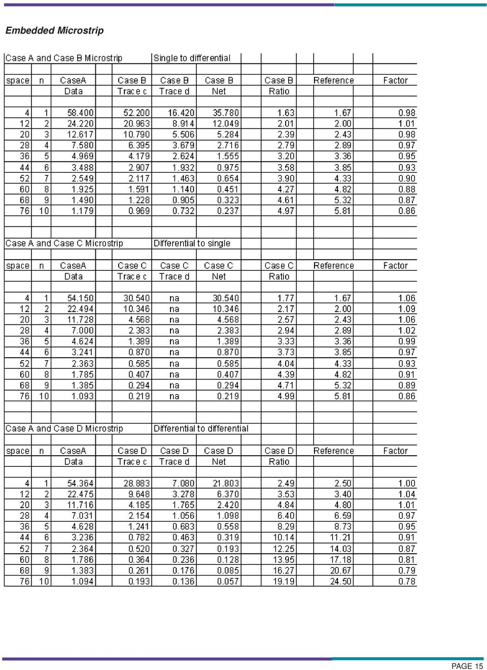
14 the left hand pair (the aggressor traces) between Figure A3 and Figure A4. This was done in every case as a control method. Finally, the driver for the aggressor trace(s) was always a DS90LV031ATM, a standard model supplied with the Hyperlynx tool set. There was no specific reason for selecting this driver over any other. The rise time of this driver is very approximately 2 nsec when the "Fast-Strong" simulation option is selected. Figure A5 - Typical simulation showing the aggressor signals. represents Case D, a differential aggressor driving a differential victim pair. Note in Figure A5 the crosstalk coupled signals are barely visible along the centerline of the scope display. Figure A6 illustrates the crosstalk signals. The blue trace represents the crosstalk coupled noise on a single-ended victim from a single-ended aggressor, the control case. The yellow and violet traces are the signals on the individual traces of the differential victim pair. The hypothesis under study in the paper suggests that the common mode part of these signals is not important, just the differential mode component is important. The differential mode component of the signal is the difference between these two traces. (In the case of a single-ended victim, there would only be the single yellow trace for that signal.) The raw data is provided in the tables in Appendix 2. The first column corresponds to the edge-to-edge spacing between Trace b and Trace c in the model. The second column provides the value for the variable "n" that corresponds to this spacing. The third data column is the coupled noise from a single-ended aggressor (Trace b) to a single-ended victim (Trace c). It is recorded in each investigation as a control. The next two data columns record the data on the victim trace(s) and the "net" column is the net differential signal on the victim trace(s). The absolute value of these readings (data) has little meaning. It is the relationship between the various data points that is meaningful. The "ratio" column records the calculated ratio of the case under test to Case A. The reference column is the expected ratio, based on, and recorded from, Table 1 in the paper. The "factor" column is the ratio of the calculated ratio to the expected ratio. Footnotes for the Appendix A1. See "Crosstalk, Parts 1 and 2," available at Figure A6 - The coupled crosstalk signals from the model shown in Figure A5. Figure A5 and Figure A6 illustrate a typical model simulation result. Figure A5 illustrates the aggressor signals. The orange trace is the single-ended aggressor driving coupled to a single-ended victim (Case A). This is a "control" signal used in every model simulation. The red trace is the aggressor signal under evaluation. It may be a single-ended signal or (part of) a differential signal, depending on the case. In the specific case shown in Figure A5 the red trace PAGE 13

15 APPENDIX 2 - RAW DATA FROM THE MODELS Microstrip PAGE 14

16 Embedded Microstrip PAGE 15

17 Balanced Stripline PAGE 16

18 Asymmetric Stripline PAGE 17

19 ABOUT THE AUTHOR Douglas Brooks has a BS and an MS in Electrical Engineering from Stanford University and a PhD from the University of Washington. During his career has held positions in engineering, marketing, and general management with such companies as Hughes Aircraft, Texas Instruments and ELDEC. Brooks has owned his own manufacturing company, and he formed UltraCAD Design Inc. in UltraCAD is a service bureau in Bellevue, WA, that specializes in large, complex, high density, high-speed designs, primarily in the video and data processing industries. Brooks has written numerous articles through the years, including articles and a column for Printed Circuit Design magazine. Prentice Hall published his book Signal Integrity Issues and Printed Circuit Board Design in He has been a frequent seminar leader at PCB Design Conferences, and has presented seminars around the world, including Moscow, China, Japan, and Taiwan. His primary objective in his speaking and writing has been to make complex issues easily understandable to those individuals without a technical background. You can visit his web page at and e- mail him at doug@ultracad.com. For more information, call us or visit: Copyright 2004 Mentor Graphics Corporation. This document contains information that is proprietary to Mentor Graphics Corporation and may be duplicated in whole or in part by the original recipient for internal business purposed only, provided that this entire notice appears in all copies. In accepting this document, the recipient agrees to make every reasonable effort to prevent the unauthorized use of this information. Mentor Graphics is a registered trademark of Mentor Graphics Corporation. All other trademarks are the property of their respective owners. Corporate Headquarters Mentor Graphics Corporation 8005 S.W. Boeckman Road Wilsonville, Oregon USA Phone: Silicon Valley Headquarters Mentor Graphics Corporation 1001 Ridder Park Drive San Jose, California USA Phone: Fax: Europe Headquarters Mentor Graphics Corporation Deutschland GmbH Arnulfstrasse Munich Germany Phone: Fax: Pacific Rim Headquarters Mentor Graphics (Taiwan) Room 1603, 16F, International Trade Building No. 333, Section 1, Keelung Road Taipei, Taiwan, ROC Phone: Fax: Japan Headquarters Mentor Graphics Japan Co., Ltd. Gotenyama Hills 7-35, Kita-Shinagawa 4-chome Shinagawa-Ku, Tokyo 140 Japan Phone: Fax: JC Printed on Recycled Paper TECH6650-w PAGE 18