Linköping University Electronic Press

Transcription

1 Linköping University Electronic Press Report Well-posed boundary conditions for the shallow water equations Sarmad Ghader and Jan Nordström Series: LiTH-MAT-R, , No. 4 Available at: Linköping University Electronic Press

2 Generated using version 3. of the official AMS L A TEX template Well-posed boundary conditions for the shallow water equations Sarmad Ghader Department of Space Physics, Institute of Geophysics, University of Tehran, Tehran, Iran Jan Nordström Division of Computational Mathematics, Department of Mathematics, Linköping University, SE Linköping, Sweden Corresponding author address: Sarmad Ghader, Institute of Geophysics, University of Tehran, North Karegar Ave., Tehran, Iran. sghader@ut.ac.ir 1

3 ABSTRACT We derive well-posed boundary conditions for the two-dimensional shallow water equations by using the energy method. Both the number and the type of boundary conditions are presented for subcritical and supercritical flows on a general domain. Then, as an example, the boundary conditions are discussed for a rectangular domain. 1

4 1. Introduction The single layer shallow water models are extensively used in numerical studies of large scale atmospheric and oceanic motions. This model describes a fluid layer of constant density in which the horizontal scale of the flow is much greater than the layer depth. The dynamics of the single layer model is of course less general than three dimensional models, but is often preferred because of its mathematical and computational simplicity (e.g., Pedlosky (1987); Vallis (006)). Well-posed boundary conditions are an essential requirement for all stable numerical schemes developed for initial boundary value problems. For the one-dimensional shallow water equations, well-posed boundary conditions have been derived previously by transforming them into a set of decoupled scalar equations (e.g., Durran (010)), but the two-dimensional case is more complicated. Although significant computational efforts have been spent on the shallow water equations (e.g., Lie (001); Mcdonald (00, 003); Brown and Gerritsen (006); Voitus et al. (009)), a complete derivation of multi-dimensional well-posed boundary conditions is still lacking. This work is devoted to the assessment of well-posedness and derivation of boundary conditions for the two-dimensional shallow water equations. The core mathematical tool used in this study is the energy method where one bounds the energy of the solution by choosing a minimal number of suitable boundary conditions (e.g., Gustafsson et al. (1995); Nordström and Svärd (005); Gustafsson (008)). The remainder of this paper is organized as follows. The shallow water equations are given in section. Section 3 gives the various definitions of well posedness. In section 4 well posed boundary conditions for the two dimensional shallow water equations for a general domain are derived. The boundary conditions for a rectangular domain, as an example, are presented and discussed in section 5. Finally, concluding remarks are given in section 6.

5 . The shallow water equations The inviscid single-layer shallow water equations, including the Coriolis term, are (e.g., Vallis (006)) DV Dt + f ˆk V + g h = 0 (1) Dh + h V Dt = 0 () where V = uî+vĵ is the horizontal velocity vector with u and v being the velocity components in x and y directions, respectively. î and ĵ are the unit vectors in x and y directions, respectively. h represents the surface height, D()/Dt = ()/ t + (v )() is the substantial time derivative, f is the Coriolis parameter and g is the acceleration due to gravity. The unit vector in vertical direction is denoted by ˆk. Here, we use the f-plane approximation where the Coriolis parameter is taken to be a constant. a. The linearized two-dimensional shallow water equations The vector form of the two-dimensional shallow water equations, linearized around a constant basic state, can be written as u t + Au x + Bu y + Cu = 0 (3) where the subscripts t, x and y denote the derivatives. The definition of the vector u and the matrices A, B and C is u U 0 g u = v, A = 0 U 0 H 0 U h, B = V V g 0 H V, C = 0 f 0 f Here, u and v are the perturbation velocity components and h is the perturbation height. In addition, U, V and H represent the constant mean fluid velocity components and height. 3

6 3. Well-posedness Before embarking on the derivation of well posed boundary conditions of the shallow water equations, we need to define well posedness. Consider the initial boundary value problem q t = Pq + F, x Ω, t 0 Lq = g, x Ω, t 0 (4) q = f, x Ω, t = 0 where q is the solution, x is the space vector, P is a spatial differential operator and L is the boundary operator. F is a forcing function, g and f are boundary and initial functions, respectively. F, g and f are the known data of the problem. We need the following definition. Definition 1. Consider the problem (4). The differential operator P is called semi-bounded if for all q V, where V being the space of differentiable functions satisfying the boundary conditions Lq = 0, the inequality (q, Pq) α q (5) holds. In (5), α is a constant independent of q. Here, (, ) and denote the scalar product and norm, respectively. The estimate (5) guarantees that an energy estimate exists for (4). However, to many boundary conditions could have been used, which means that no solution exist. To guarantee existence, we also need the following definition. Definition. The differential operator P is maximally semi-bounded if it is semi-bounded in the function space V but not semi-bounded in any space with fewer boundary conditions. Finally, the following theorem relates maximal semi-boundedness and well posedness. Theorem 1. Consider the initial boundary value problem (4). If the operator P is maximally semi-bounded, then the initial boundary value problem with g = 0 is well posed. 4

7 More details on these definitions, theorem and proofs are given by Gustafsson et al. (1995) and Gustafsson (008). As will be shown below, we will follow the path set by others and perform the analysis on the linearized constant coefficient problem. This is no limitation since it can be shown that if the constant coefficient and linearized form of an initial boundary value system is well-posed then the associated original nonlinear problem is also well posed. For more details, see the linearization and localization principles in Kreiss and Lorenz (1989). 4. Well-posedness of the shallow water equations The linearized constant coefficient two-dimensional shallow water equations (3) with initial and boundary conditions can be formulated as u t + Au x + Bu y + Cu = 0 (x, y) Ω, t 0 (6) Lu(x, y, t) = g(x, y, t), (x, y) Ω, t 0 (7) u(x, y, 0) = f(x, y), (x, y) Ω, t = 0 (8) where f is the initial data and g the boundary data. L is the boundary operator, and will be the main focus in this paper. To be able to integrate by parts we need to symmetrize the equations (Abarbanel and Gottlieb 1981; Nordström and Svärd 005). Therefore, equation (6) is rewritten as: (Su) t + SAS 1 (Su) x + SBS 1 (Su) y + SCS 1 (Su) = 0. (9) In (9), S is symmetrizing matrix. The matrices A s = SAS 1 and B s = SBS 1 must be symmetric and we find that A s = U 0 c 0 U 0 c 0 U, Bs = V V c 0 c V 5

8 where c = gh is the gravity wave speed and C s = SCS 1 = C. The new variable which transforms equation (6) to a symmetric form is found as v = Su = (u, v, gh /c) T, where the superscript T denotes transpose. Therefore, equation (6) is transformed to v t + A s v x + B s v y + Cv = 0. (10) The following definition of scalar product and norm for functions will be used (u, v) = uvdxdy, u = (u, u). Ω Multiplying equation (10) by v T followed by integration over the domain leads to v t + (v T A s v) x dxdy + (v T B s v) y dxdy = 0. (11) Ω Ω The term containing C, due to its skew-symmetry, is zero. Using Gauss theorem on equation (11) we find v t + (v T Âv)ds = 0. (1) Ω In (1), Â = ˆn (As, B s ), ˆn = (n x, n y ) = (dy, dx)/ds is the outward pointing unit vector on the surface Ω and ds = dx + dy. After finding the eigenvalues of Â, the right eigenvectors can be used to write Λ = R T ÂR (13) where R = nx n y n x n y n x n y 1 1 0, Λ = ω c ω ω + c. (14) 6

9 In (14), ω = n x U + n y V = (U, V ) ˆn. Using the new variable w = R T v, equation (1) is rewritten as v t + w T Λwds = 0. (15) Ω Equation (15) implies that the two-dimensional shallow water equations will be wellposed and v bounded if the surface integral in (15) is positive. Consequently, condition (15) can be used to find well-posed boundary conditions. a. Well-posed boundary conditions for a general domain The sign of ω = (U, V ) ˆn determines whether we have inflow or outflow. In other words, ω < 0 signals inflow and ω > 0 outflow. In addition we have w T Λw = w 1(ω c) + w ω + w 3(ω + c) (16) where w 1 = (gh c (u, v ) ˆn), w = (u, v ) ˆn, w 3 = (gh c + (u, v ) ˆn) To find well-posed boundary conditions for a general domain, condition (15) implies that w T Λw 0 (17) is necessary at both inflow and outflow boundaries. In addition, it should be noted that based on definition and theorem 1 (see section 3), for well-posedness we need to satisfy condition (17) with a minimal number of boundary conditions. For subcritical inflow where ω < c, the components of the diagonal matrix Λ are ω < 0, ω c < 0 and ω + c > 0. At a subcritical outflow boundary the components of the diagonal matrix Λ are ω > 0, ω c < 0 and ω + c > 0. Therefore, for the subcritical case we need two boundary conditions at the inflow boundary and one boundary condition at the outflow boundary. This choice makes the spatial operator maximally semi-bounded, and well-posedness follows (see section 3). 7

10 For supercritical inflow where ω > c, the components of the diagonal matrix Λ are ω < 0, ω c < 0 and ω + c < 0. At the outflow boundary, the components of the diagonal matrix Λ are ω > 0, ω c > 0 and ω + c > 0. For this case, we need three boundary conditions at an inflow boundary and none at an outflow boundary. 1) Subcritical inflow and outflow boundaries The two boundary conditions for the inflow case that assure that all terms in condition (17) are positive are w = 0, w 1 β i w 3 = 0. (18) By substituting (18) into (17), we find that the coefficient β i must satisfy c + ω β i c ω. Note that β i 1 and the extreme values ±1 are only attained for ω = 0. For a subcritical outflow boundary only one boundary condition is needed in order to satisfy condition (17). To assure that all terms are positive we need w 1 β o w 3 = 0. (19) By substituting (19) into (17), we find that the coefficient β o must satisfy c + ω β o c ω. Here, β o 1 and the extreme values ±1 are obtained for ω = 0. Since β o 1, the special choices w 1 w 3 = 0, or w 1 + w 3 = 0 (0) are valid boundary conditions. The boundary condition (19) is more general but the specific boundary conditions (0) are less complex and easier to implement. The boundary conditions (0) expressed in primitive variables are (u, v ) ˆn = 0 and h = 0, respectively. In addition, it can be seen that when ω goes towards zero, the subcritical inflow and outflow boundary conditions smoothly transient to each other. 8

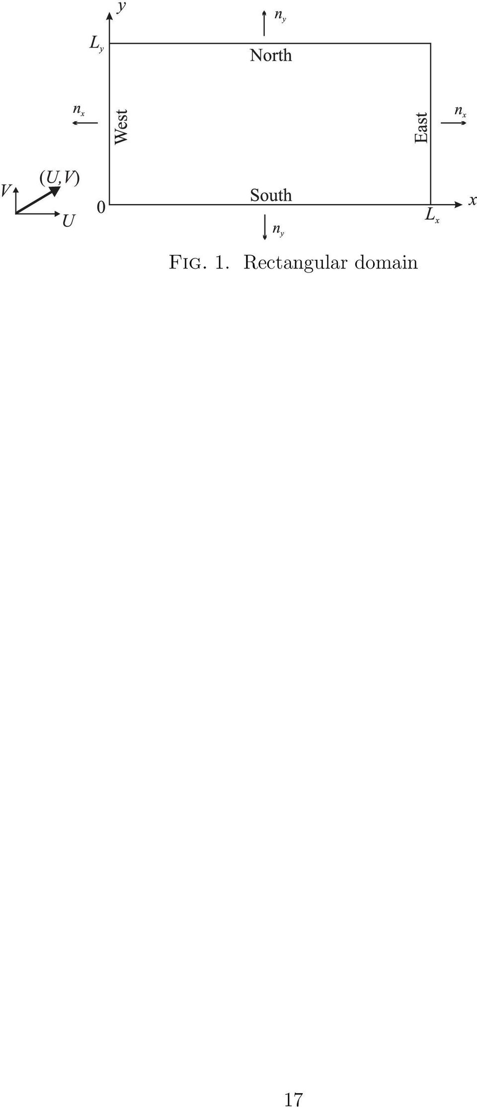
11 ) Supercritical inflow and outflow boundaries For the supercritical inflow boundary we need three boundary conditions to satisfy condition (17). They are w 1 = w = w 3 = 0. (1) Condition (17) is automatically satisfied at a supercritical outflow boundary and therefore no boundary conditions are needed in that case. b. The boundary conditions for the nonlinear problem The homogeneous boundary conditions derived above will be used for the nonlinear shallow water equations by augmenting them with known data at boundaries. For example, at the inflow boundary in the subcritical case, the boundary conditions (18) for the nonlinear problem have the following form w = g 1, w 1 β i w 3 = g () where g 1 = w e and g = w 1e β i ew 3e, respectively. The subscript e denotes known data at the boundary Ω. The boundary conditions for the other cases are found in the same way. 5. The boundary conditions for a rectangular domain In this section the general well-posed boundary conditions derived above are considered for a specific rectangular domain, which can be considered as a representative geometry used in real world two dimensional limited area models, see Figure 1. It is assumed that the basic state velocity components are positive (U > 0, V > 0). By this assumption, it can be seen that the west (x = 0, 0 y L y ) and south (y = 0, 0 x L x ) boundaries are of inflow type since ω < 0. The east (x = L x, 0 y L y ) and north (y = L y, 0 x L x ) boundaries are of outflow type since ω > 0. Note that the 9

12 crucial parameter which decides whether the flow is subcritical or supercritical is ω, not the magnitude of the vector (U, V ). a. Subcritical inflow boundaries We start with the south boundary where ˆn = (0, 1) and we have w T Λw = w 1(ω c) + w ω + w 3(ω + c) (3) where ω = V, V < c and w 1 = (gh c + v ), w = u, w 3 = (gh c v ). At an inflow boundary we need two boundary conditions and it can be seen that these two boundary conditions will have the following form using equation (18) u = 0, gh c + v β i ( gh c v ) = 0. (4) The coefficient β i is bounded by (c V )/(c + V ). We can find well-posed boundary conditions for the west boundary in a similar way. For the west boundary ˆn = ( 1, 0) and we have w T Λw = w 1(ω c) + w ω + w 3(ω + c) (5) where ω = U, U < c and w 1 = (gh c + u ), w = v, w 3 = (gh c u ). Therefore, the boundary conditions for the west boundary are found as v = 0, gh c + u β i ( gh c u ) = 0 (6) where the coefficient β i is bounded by (c U)/(c + U). 10

13 b. Subcritical outflow boundaries We start with the east boundary where ˆn = (1, 0) and we have w T Λw = w 1(ω c) + w ω + w 3(ω + c) (7) where ω = U, U < c and w 1 = (gh c u ), w = v, w 3 = (gh c + u ). For the subcritical outflow boundary we can find the boundary condition from (19) which becomes gh c u β o ( gh c + u ) = 0. (8) The coefficient β o is bounded by (c + U)/(c U). If we choose the extreme values β o = 1 or β o = 1, the boundary condition given by (8) will be reduced to u = 0, or h = 0. (9) Similarly, at the north boundary ˆn = (0, 1) and w T Λw = w 1(ω c) + w ω + w 3(ω + c) (30) where ω = V, V < c and w 1 = (gh c v ), w = u, w 3 = (gh c + v ) Then, the boundary condition (19) for this boundary leads to gh c v β o ( gh c + v ) = 0 (31) where the coefficient β o is bounded by (c + V )/(c V ). Here, if we use extreme values β o = 1 or β o = 1, the boundary condition (31) will be reduced to v = 0, or h = 0. (3) 11

14 c. Supercritical inflow and outflow boundaries For the supercritical case we need three boundary conditions at inflow. For this case equation (1) reads u = v = h = 0. (33) No boundary conditions are needed at the supercritical outflow boundaries. 6. Concluding remarks We have derived well-posed boundary conditions for the linearized two-dimensional shallow water equations by using the energy method. Well-posed boundary conditions including the type and number of boundary conditions have been derived for subcritical and supercritical inflow and outflow boundaries on a general two dimensional domain. For the subcritical inflow case it was shown that we need two boundary conditions to bound the energy of the solution and at the subcritical outflow boundary only one boundary condition is needed. For the supercritical inflow case it was shown that three boundary conditions are required and at the outflow boundary none. The exact form of the boundary operator was determined for all four cases. In addition, as an example, a rectangular domain was considered and the specific wellposed boundary conditions at the inflow and outflow boundaries were extracted. The next stage of the present work is to implement the derived well-posed boundary conditions in a numerical algorithm. We will use high order finite difference approximations with summation by parts operators and weak boundary procedures to implement the different types of boundary conditions derived in this paper. Acknowledgments. Authors would like to thank universities of Tehran and Linköping for supporting this 1

15 research work. 13

16 REFERENCES Abarbanel, S. and D. Gottlieb, 1981: Optimal time splitting for two- and three-dimensional Navier-Stokes equations with mixed derivatives. Journal of Computational Physics, 41, Brown, M. and M. Gerritsen, 006: An energy-stable high-order central difference scheme for the two-dimensional shallow water equations. Journal of Scientific Computing, 8, Durran, D. R., 010: Numerical methods for fluid dynamics with applications to geophysics. Springer, 516 pp. Gustafsson, B., 008: High order difference methods for time dependent PDE. Springer, 334 pp. Gustafsson, B., H. O. Kreiss, and J. Oliger, 1995: Time dependent problems and difference methods. John Wiley and Sons, 64 pp. Kreiss, H. O. and J. Lorenz, 1989: Initial boundary value problems and the Navier-Stokes equations. Academic Press, 40 pp. Lie, I., 001: Well-posed transparent boundary conditions for the shallow water equations. Applied Numerical Mathematics, 38, Mcdonald, A., 00: A step toward transparent boundary conditions for meteorological models. Mon. Wea. Rev., 130, Mcdonald, A., 003: Transparent boundary conditions for the shallow-water equations: Testing in a nested environment. Mon. Wea. Rev., 131,

17 Nordström, J. and M. Svärd, 005: Well posed boundary conditions for the Navier-Stokes equations. SIAM J. Numer. Anal., 43, Pedlosky, J., 1987: Geophysical fluid dynamics. Springer-Verlag, 710 pp. Vallis, G. K., 006: Atmospheric and oceanic fluid dynamics: Fundamentals and large-scale circulation. Cambridge University Press, 745 pp. Voitus, F., P. Termonia, and P. Benard, 009: Well-posed lateral boundary conditions for spectral semi-implicit semi-lagrangian schemes: tests in a one-dimensional model. Mon. Wea. Rev., 137,

18 List of Figures 1 Rectangular domain 17 16

19 Fig. 1. Rectangular domain 17