Descriptive statistics Statistical inference statistical inference, statistical induction and inferential statistics
|
|
|
- Valentine Poole
- 9 years ago
- Views:
Transcription
1 Descriptive statistics is the discipline of quantitatively describing the main features of a collection of data. Descriptive statistics are distinguished from inferential statistics (or inductive statistics), in that descriptive statistics aim to summarize a sample, rather than use the data to learn about the population that the sample of data is thought to represent. This generally means that descriptive statistics, unlike inferential statistics, are not developed on the basis of probability theory. Statistical inference is the process of drawing conclusions from data that is subject to random variation, for example, observational errors or sampling variation. More substantially, the terms statistical inference, statistical induction and inferential statistics are used to describe systems of procedures that can be used to draw conclusions from datasets arising from systems affected by random variation, such as observational errors, random sampling, or random experimentation. Initial requirements of such a system of procedures for inference and induction are that the system should produce reasonable answers when applied to well-defined situations and that it should be general enough to be applied across a range of situations.

2 Unit: A single entity of statistical interests Population: A complete set of collection of unit. Statistical population: The set of all measurements. Sample: A subset from the statistical population A good sample should be randomized and is representative of the population while a bad sample contains subjectivity and is biased.

3 Descriptive measures of a statistical sample (or population) computed from the data. Given data, x 1, x 2,, x i,, x n the most standard measures are: Sample mean (often simply called the mean) is the average value x = Median describes the center of the data set when the data is ordered by value If n is an odd number, there is exactly one data value lying at the center of the ordered data values. It is the k th data value where k = (n+1)/2. In this case the median value is x k If n is an even number, there are two values lying at the center of the ordered data values. Those are the k th and k+1 st values where k = n/2. In this case the median value is defined as n i=1 n x i x k + x k+1 2
/2. In this case the median value is x k If n is an even number, there are two values lying at the center of the ordered data values.")
4 Variance and Standard Deviation: In addition to knowing the average behavior (value) of a set of data, we would like to know how much the data is spread about the average. This is computed by deviations from the mean Let x be the mean value of the data x 1, x 2,, x i,, x n The differences, x 1 x, x 2 x,, x i x,, x n x are called the deviations from the mean The sum of the deviations n x i x i=1 = 0 (i.e. the sum of the positive deviations exactly cancels the sum of the negative deviations.) This is one of the nice properties of the mean. Summing the squares of the deviations gives a non-zero result which gives a useful measure of the spread of the data about the mean. The common measure for this spread is the sample variance, s 2 s 2 = n x i x 2 i=1 n 1 Since the deviations sum to 0, the value of 1 of them can always be calculated from the other n 1. Therefore only n 1 of the deviations are independent, explaining the n 1 (instead of n) appearing in the denominator of s 2

5 Since the units of the sample variance are the square of the units of the data, we define the sample standard deviation s = n i=1 n 1 x i x 2 If the deviations from the mean are generally large, the standard deviation will be large. If the deviations from the mean are generally small, the standard deviation will be small. When do we know the standard deviation is large? Is s = 1.67 large or small? That depends on the mean value. Thus we use the fraction relative variation, s x or the percent coefficient of variation, V = s x 100% to quantify the size of the standard deviation. e.g. a set of measurements made with micrometer s A and B give the following table of results. Which micrometer measurements are more accurate? Micrometer mean std dev coef of var A 3.92 mm mm 0.39% B 1.54 in in 0.56%

6 Alternate way to compute sample variance s 2 n x i x 2 i=1 n 1 = n x i 2 i=1 nx 2 n 1 Operations count + n-1 n-1 n+1 2 n n Total 3n+1 2n+4 more efficient on a computer hand calculator

7 Example: meals served over 5 weeks: n = 5, mean number meals served is x = = 14.2 the ordered data is median value of meals served is given by the k th data value where k = (n+1)/2 = 6/2 = 3 That is median = x 3 = 14 e.g. In the alloy strength data, n = 58. The mean value of alloy strength is x = 70.7 To compute the median value with n even, we want the k = 58/2 = 29 th and k + 1 = 30 th values in the ordered data array. From the stem-leaf display, these two values are rapidly found to be 70.5 and Therefore, the median value of alloy strength is ( )/2 = 70.55

8 Except in very special cases, the mean and median values are NOT the same. Mean values are very susceptible to outlier values, median values are not. e.g. reconsider the meals per week data: The mean value is x = 14.2; the median value is 14. Suppose the last value is changed from 27 to 67, giving the data set The mean value is now x = 22.2; the median value is unchanged at 14. The mean is the most common single number used to discribe the average behavior of a data set. This is commonly misinterpreted to also be the central behavior of the data set. Except in special cases to be discussed later in the course, the mean does not characterize the central behavior of the data set. If you want to know the central behavior of the data, use the median. e.g. if you are told that the average grade on an exam is 77.6, does that mean half of the class scored above 77.6?

9 Computing mean and sample variance from data with repetition Consider the data set: 7.6, 7.6, 7.7, 7.7, 7.7, 7.7, 7.8, 7.8, 7.8, 7.9 The mean value is x = = Therefore, if a data set consists of n values, but only k < n of the values are different, where the value x i occurs g i times then Similarly, for variance: x = k i=1 n x i g i s 2 = k i=1 g i (x i x ) 2 n 1
 2 n 1")
10 Consider Sample Data: compressive strength measurements of 58 samples of an aluminum alloy 66.4, 67.7, 68.0, 68.0, 68.3, 68.4, 68.6, 68.8, 68.9, 69.0, 69.1, 69.2, 69.3, 69.3, 69.5, 69.5, 69.6, 69.7, 69.8, 69.8, 69.9, 70.0, 70.0, 70.1, 70.2, 70.3, 70.3, 70.4, 70.5, 70.6, 70.6, 70.8, 70.9, 71.0, 71.1, 71.2, 71.3, 71.3, 71.5, 71.6, 71.6, 71.7, 71.8, 71.8, 71.9, 72.1, 72.2, 72.3, 72.4, 72.6, 72.7, 72.9, 73.1, 73.3, 73.5, 74.2, 74.5, 75.3

11 Estimating mean and sample variance from a frequency distribution Suppose the original data is lost and all you have is the frequency distribution You can approximate the computation of the sample mean and variance using x s 2 k i=1 n x i f i where x i are the bin marks f i are the bin frequencies k is the number of bins (9 in the example table) and n = k k i=1 f i (x i x ) 2 f i n 1 Alloy Strength Bin Bin Mark Frequency x i ( ] ( ] ( ] ( ] ( ] ( ] ( ] ( ] ( ] i=1 is the number of data points (58 in the example table) f i
![example table) and n = k k i=1 f i (x i x ) 2 f i n 1 Alloy Strength Bin Bin Mark Frequency x i (66.3 67.3] 66.8 1 (67.3 68.3] 67.8 4 (68.3 69.3] 68.8 9 (69.3 70.](/docs-images/47/19926576/images/page_11.jpg "3] 69.8 13 (70.3 71.3] 70.8 11 (71.3 72.3] 71.8 10 (72.3 73.3] 72.8 6 (73.3 74.3] 73.8 2 (74.3 75.3] 74.")
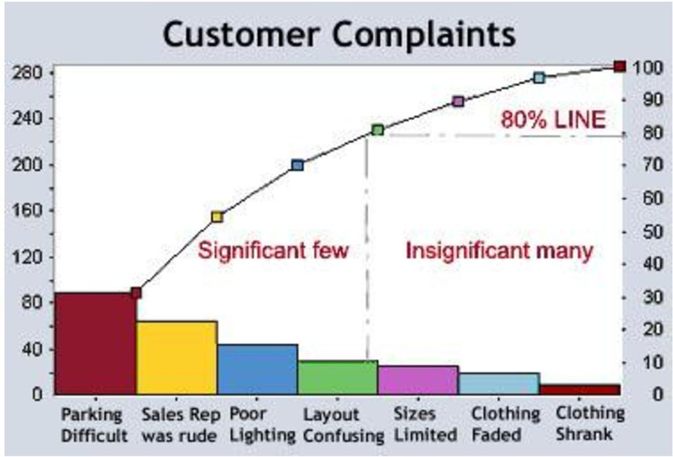
, is a type of chart that contains both bars and a line graph, where")

12 A Pareto chart, named after Vilfredo Pareto ( , was an Italian engineer, sociologist, economist, political scientist and philosopher), is a type of chart that contains both bars and a line graph, where individual values are represented in descending order by bars, and the cumulative total is represented by the line. Pareto s empirical law: any assortment contains a few major components and many minor components.

13
14 Pareto diagrams: Pareto diagrams are bar charts that show the percentage of the total response variance attributable to each factor and interaction.

15 Wilkinson dot plots: as a representation of a distribution consists of group of data points plotted on a simple scale.

16 Cleveland dot plots: refer to plots of points that each belong to one of several categories. They are an alternative to bar charts or pie charts, and look somewhat like a horizontal bar chart where the bars are replaced by a dots at the values associated with each category.

17 Sample Data: compressive strength measurements of 58 samples of an aluminum alloy 66.4, 67.7, 68.0, 68.0, 68.3, 68.4, 68.6, 68.8, 68.9, 69.0, 69.1, 69.2, 69.3, 69.3, 69.5, 69.5, 69.6, 69.7, 69.8, 69.8, 69.9, 70.0, 70.0, 70.1, 70.2, 70.3, 70.3, 70.4, 70.5, 70.6, 70.6, 70.8, 70.9, 71.0, 71.1, 71.2, 71.3, 71.3, 71.5, 71.6, 71.6, 71.7, 71.8, 71.8, 71.9, 72.1, 72.2, 72.3, 72.4, 72.6, 72.7, 72.9, 73.1, 73.3, 73.5, 74.2, 74.5, 75.3 Dot diagram: each data value represented as a point, with care taken so that points with the same value do not overlap Youtube teaching page: Or search dot plot statstics

18 A dot chart or dot plot is a statistical chart consisting of data points plotted on a simple scale, typically using filled in circles. There are two common, yet very different, versions of the dot chart. The first is described by Wilkinson as a graph that has been used in hand-drawn (pre-computer era) graphs to depict distributions. The other version is described by Cleveland as an alternative to the bar chart, in which dots are used to depict the quantitative values (e.g. counts) associated with categorical variables. Data assessment through visualization - outliers - differences between sets of samples Production A Production B

19 Frequency Distributions (Tables) Look at frequency of distribution of data over subintervals (bins, classes) spanning the entire range of data Alloy Strength Subinterval Frequency Relative Percent Cumulative Frequency Frequency Frequency ( ] ( ] ( ] ( ] ( ] ( ] ( ] ( ] ( ] Total
![72 1 (67.3 68.3] 4 0.0690 6.90 5 (68.3 69.3] 9 0.1552 15.52 13 (69.3 70.3] 13 0.2241 22.41 26 (70.3 71.3] 11 0.1897 18.97 37 (71.](/docs-images/47/19926576/images/page_19.jpg "3 72.3] 10 0.1724 17.24 47 (72.3 73.3] 6 0.1034 10.34 53 (73.3 74.3] 2 0.0345 3.45 56 (74.3 75.3] 2 0.0345 3.45 58 Total 58 1.")
20 Histogram: Frequency Distribution: number n i of data values in bin i Relative Frequency Distribution: relative number n i / n of data values in bin i (n is the total number of data values) Percent Frequency Distribution: percent ( (n i / n)*100 ) of data values in bin i Cumulative Distribution: Total number of data values up to and including bin i i j=1 n j Note: Bins must not overlap Bins must accommodate all data Bins should be of the same width

21 Frequency Distribution Decisions number of bins & bin width Goals - enough ( ) data values in most bins - enough bins ( 10) to see shape of distribution If the data set is small (< 100), the number of bins and amount of data per bin will be reduced from the optimum goals. Aim for 5 bins. strength data: 58 values from 66.4 to bins over the range 66.3 to 75.3 gives a bin width of ( )/9 = 1.0 with an average frequency of 58/9 = 6.4 data values per bin. bin ranges must respect data accuracy e.g. (66.3, 67.3], (67.3, 68.3] if data is given to tenths values (1 decimal place) (65, 67], (67, 69] if data is given only to ones value (no decimal places) numerical assignment to bin each data value must be uniquely assigned to a single bin ( ] convention (66.3, 67.3] data value 67.3 assigned to bin 1 (67.3, 68.3] [ ) convention [66.3, 67.3) [67.3, 68.3) data value 67.3 assigned to bin 2
22 The textbook adopts the following notation for bins (classes) Class limits (or class boundaries) the endpoints of each bin interval Class mark the midpoint of each bin Class interval the common width of each bin = the distance between class marks This notation is not necessarily standard.
23 Frequency Histograms (plotting frequency distributions) Frequency plot using class marks
24 Relative frequency plot with cumulative distribution
25 Density distributions A density distribution is a frequency distribution for which height of bin i = relative frequency of bin i width of bin i The area of each bin i = the relative frequency for bin i The total area of a density distribution is always unity ( = 1 ) ONLY with density distributions are bins of different widths permissible (although different bin widths should still be avoided when possible)
26 Note: if the bin limits remain the same, the shape of the distribution (frequency, relative frequency, density) remains unchanged.
27 Quartiles and Percentiles In the same way that we use the median to find the center point of a data set ½ of the data values lie below the median, ½ of the values lie above we can fine the first quartile Q 1, the data value that has ¼ of the data points lying below it (and 1 ¼ = ¾ of the points lying above it). Since ¼ of the data corresponds to 25% of the data, Q 1 is also referred to as the 25 th percentile P 0.25 of the data set. We can generalize this to the 100 p th percentile P 0.p, the data value that has 100 p% of the data points lying below it (and 100 (1 p) % of the data points lying above it). The 50 th percentile P 0.50 is known as the second quartile Q 2 and is, in fact, identical to the median of the data set. The 75 th percentile P 0.75 is known as the third quartile Q 3. To compute percentile P 0.p in a data set of n values: 1. order the data smallest to largest 2. compute the product n p if np is not an integer, round it up to the next integer value and find the corresponding data point if np is an integer k, take the average of the k th and (k+1) st data values.
28 e.g. The Q 1, Q 3 and Q 3 values for the alloy strength data set are: Q 1 (p = 0.25) np = = 14.5 round to 15. From the Stem-Leaf table, Q 1 = x 15 = 69.4 Q 2 (p = 0.50) np = = 29 Average the 29 th and 30 th values. From the Stem- Leaf table, Q 2 = (x 29 + x 30 ) /2 = ( )/2 = as previous computed for the median value of this data set Q 3 (p = 0.75) np = = 43.5 round to 44. From the Stem-Leaf table, Q 3 = x 44 = 71.8 As previously implied, the range of the data is range = maximum minimum = x n x 1 when the data are ordered smallest to largest The middle half of the data lies in the interquartile range interquartile range = Q 3 Q 1 e.g. The range for the alloy strength data set is = 8.9 The interquartile range is Q 3 Q 1 = = 2.4
29 Unlike the dot diagram, which displays every value, frequency distributions suppress information on individual data values. Stem-Leaf displays provide a tabular way of organizing the display of all data values stem labels leaf entries are comprised leaf of the last digit of the data 58 values leaf count to check no data lost
30 Stem-Leaf displays are a useful way to analyze class grades, especially for computing median and quartile values
31 Boxplots: (aka box-whisker plot) plot quartile information Q 1 Q 2 Q 3 whisker extending to minimum data value whisker extending to maximum data value
32 Boxplot variation: 1.5 x IQ distance IQ distance 1.5 x IQ distance Q 1 Q 2 Q 3 whisker extending to smallest data value lying above Q 1 IQ distance whisker extending to largest data value lying below Q 3 + IQ distance
33 Boxplot combined with sample mean and standard deviation std dev mean std dev min val Q 1 Q 2 Q 3 max val
34 Chapter 2 summary dot diagrams distributions (histograms): bins, range, bin limits, bin marks, bin interval distributions of: frequency, relative frequency, percent frequency, cumulative frequency distribution graphs, density graphs stem-and-leaf displays data quantifiers: sample mean, sample variance, sample standard deviation Quartiles, percentiles, median, interquartile range boxplots
Exploratory data analysis (Chapter 2) Fall 2011
 Fall 2011") Exploratory data analysis (Chapter 2) Fall 2011 Data Examples Example 1: Survey Data 1 Data collected from a Stat 371 class in Fall 2005 2 They answered questions about their: gender, major, year in school,
Exploratory data analysis (Chapter 2) Fall 2011 Data Examples Example 1: Survey Data 1 Data collected from a Stat 371 class in Fall 2005 2 They answered questions about their: gender, major, year in school,
Descriptive Statistics
 Y520 Robert S Michael Goal: Learn to calculate indicators and construct graphs that summarize and describe a large quantity of values. Using the textbook readings and other resources listed on the web
STATS8: Introduction to Biostatistics. Data Exploration. Babak Shahbaba Department of Statistics, UCI
 STATS8: Introduction to Biostatistics Data Exploration Babak Shahbaba Department of Statistics, UCI Introduction After clearly defining the scientific problem, selecting a set of representative members
Lecture 2: Descriptive Statistics and Exploratory Data Analysis
 Lecture 2: Descriptive Statistics and Exploratory Data Analysis Further Thoughts on Experimental Design 16 Individuals (8 each from two populations) with replicates Pop 1 Pop 2 Randomly sample 4 individuals
BNG 202 Biomechanics Lab. Descriptive statistics and probability distributions I
 BNG 202 Biomechanics Lab Descriptive statistics and probability distributions I Overview The overall goal of this short course in statistics is to provide an introduction to descriptive and inferential
Chapter 1: Looking at Data Section 1.1: Displaying Distributions with Graphs
 Types of Variables Chapter 1: Looking at Data Section 1.1: Displaying Distributions with Graphs Quantitative (numerical)variables: take numerical values for which arithmetic operations make sense (addition/averaging)
STAT355 - Probability & Statistics
 STAT355 - Probability & Statistics Instructor: Kofi Placid Adragni Fall 2011 Chap 1 - Overview and Descriptive Statistics 1.1 Populations, Samples, and Processes 1.2 Pictorial and Tabular Methods in Descriptive
2 Describing, Exploring, and
 2 Describing, Exploring, and Comparing Data This chapter introduces the graphical plotting and summary statistics capabilities of the TI- 83 Plus. First row keys like \ R (67$73/276 are used to obtain
Exercise 1.12 (Pg. 22-23)
") Individuals: The objects that are described by a set of data. They may be people, animals, things, etc. (Also referred to as Cases or Records) Variables: The characteristics recorded about each individual.
Individuals: The objects that are described by a set of data. They may be people, animals, things, etc. (Also referred to as Cases or Records) Variables: The characteristics recorded about each individual.
Pie Charts. proportion of ice-cream flavors sold annually by a given brand. AMS-5: Statistics. Cherry. Cherry. Blueberry. Blueberry. Apple.
 Graphical Representations of Data, Mean, Median and Standard Deviation In this class we will consider graphical representations of the distribution of a set of data. The goal is to identify the range of
Variables. Exploratory Data Analysis
 Exploratory Data Analysis Exploratory Data Analysis involves both graphical displays of data and numerical summaries of data. A common situation is for a data set to be represented as a matrix. There is
Chapter 2: Frequency Distributions and Graphs
 Chapter 2: Frequency Distributions and Graphs Learning Objectives Upon completion of Chapter 2, you will be able to: Organize the data into a table or chart (called a frequency distribution) Construct
Sta 309 (Statistics And Probability for Engineers)
") Instructor: Prof. Mike Nasab Sta 309 (Statistics And Probability for Engineers) Chapter 2 Organizing and Summarizing Data Raw Data: When data are collected in original form, they are called raw data. The
Instructor: Prof. Mike Nasab Sta 309 (Statistics And Probability for Engineers) Chapter 2 Organizing and Summarizing Data Raw Data: When data are collected in original form, they are called raw data. The
Exploratory Data Analysis
 Exploratory Data Analysis Johannes Schauer [email protected] Institute of Statistics Graz University of Technology Steyrergasse 17/IV, 8010 Graz www.statistics.tugraz.at February 12, 2008 Introduction
Introduction to Statistics for Psychology. Quantitative Methods for Human Sciences
 Introduction to Statistics for Psychology and Quantitative Methods for Human Sciences Jonathan Marchini Course Information There is website devoted to the course at http://www.stats.ox.ac.uk/ marchini/phs.html
The right edge of the box is the third quartile, Q 3, which is the median of the data values above the median. Maximum Median
 CONDENSED LESSON 2.1 Box Plots In this lesson you will create and interpret box plots for sets of data use the interquartile range (IQR) to identify potential outliers and graph them on a modified box
Statistics Chapter 2
 Statistics Chapter 2 Frequency Tables A frequency table organizes quantitative data. partitions data into classes (intervals). shows how many data values are in each class. Test Score Number of Students
Intro to Statistics 8 Curriculum
 Intro to Statistics 8 Curriculum Unit 1 Bar, Line and Circle Graphs Estimated time frame for unit Big Ideas 8 Days... Essential Question Concepts Competencies Lesson Plans and Suggested Resources Bar graphs
Diagrams and Graphs of Statistical Data
 Diagrams and Graphs of Statistical Data One of the most effective and interesting alternative way in which a statistical data may be presented is through diagrams and graphs. There are several ways in
Lecture 1: Review and Exploratory Data Analysis (EDA)
") Lecture 1: Review and Exploratory Data Analysis (EDA) Sandy Eckel [email protected] Department of Biostatistics, The Johns Hopkins University, Baltimore USA 21 April 2008 1 / 40 Course Information I Course
Lecture 1: Review and Exploratory Data Analysis (EDA) Sandy Eckel [email protected] Department of Biostatistics, The Johns Hopkins University, Baltimore USA 21 April 2008 1 / 40 Course Information I Course
EXAM #1 (Example) Instructor: Ela Jackiewicz. Relax and good luck!
 Instructor: Ela Jackiewicz. Relax and good luck!") STP 231 EXAM #1 (Example) Instructor: Ela Jackiewicz Honor Statement: I have neither given nor received information regarding this exam, and I will not do so until all exams have been graded and returned.
STP 231 EXAM #1 (Example) Instructor: Ela Jackiewicz Honor Statement: I have neither given nor received information regarding this exam, and I will not do so until all exams have been graded and returned.
Northumberland Knowledge
 Northumberland Knowledge Know Guide How to Analyse Data - November 2012 - This page has been left blank 2 About this guide The Know Guides are a suite of documents that provide useful information about
A Correlation of. to the. South Carolina Data Analysis and Probability Standards
 A Correlation of to the South Carolina Data Analysis and Probability Standards INTRODUCTION This document demonstrates how Stats in Your World 2012 meets the indicators of the South Carolina Academic Standards
3: Summary Statistics
 3: Summary Statistics Notation Let s start by introducing some notation. Consider the following small data set: 4 5 30 50 8 7 4 5 The symbol n represents the sample size (n = 0). The capital letter X denotes
6.4 Normal Distribution
 Contents 6.4 Normal Distribution....................... 381 6.4.1 Characteristics of the Normal Distribution....... 381 6.4.2 The Standardized Normal Distribution......... 385 6.4.3 Meaning of Areas under
MBA 611 STATISTICS AND QUANTITATIVE METHODS
 MBA 611 STATISTICS AND QUANTITATIVE METHODS Part I. Review of Basic Statistics (Chapters 1-11) A. Introduction (Chapter 1) Uncertainty: Decisions are often based on incomplete information from uncertain
Why Taking This Course? Course Introduction, Descriptive Statistics and Data Visualization. Learning Goals. GENOME 560, Spring 2012
 Why Taking This Course? Course Introduction, Descriptive Statistics and Data Visualization GENOME 560, Spring 2012 Data are interesting because they help us understand the world Genomics: Massive Amounts
Describing, Exploring, and Comparing Data
 24 Chapter 2. Describing, Exploring, and Comparing Data Chapter 2. Describing, Exploring, and Comparing Data There are many tools used in Statistics to visualize, summarize, and describe data. This chapter
Visualizing Data. Contents. 1 Visualizing Data. Anthony Tanbakuchi Department of Mathematics Pima Community College. Introductory Statistics Lectures
 Introductory Statistics Lectures Visualizing Data Descriptive Statistics I Department of Mathematics Pima Community College Redistribution of this material is prohibited without written permission of the
DESCRIPTIVE STATISTICS. The purpose of statistics is to condense raw data to make it easier to answer specific questions; test hypotheses.
 DESCRIPTIVE STATISTICS The purpose of statistics is to condense raw data to make it easier to answer specific questions; test hypotheses. DESCRIPTIVE VS. INFERENTIAL STATISTICS Descriptive To organize,
HISTOGRAMS, CUMULATIVE FREQUENCY AND BOX PLOTS
 Mathematics Revision Guides Histograms, Cumulative Frequency and Box Plots Page 1 of 25 M.K. HOME TUITION Mathematics Revision Guides Level: GCSE Higher Tier HISTOGRAMS, CUMULATIVE FREQUENCY AND BOX PLOTS
Week 1. Exploratory Data Analysis
 Week 1 Exploratory Data Analysis Practicalities This course ST903 has students from both the MSc in Financial Mathematics and the MSc in Statistics. Two lectures and one seminar/tutorial per week. Exam
Summary of Formulas and Concepts. Descriptive Statistics (Ch. 1-4)
") Summary of Formulas and Concepts Descriptive Statistics (Ch. 1-4) Definitions Population: The complete set of numerical information on a particular quantity in which an investigator is interested. We assume
Summary of Formulas and Concepts Descriptive Statistics (Ch. 1-4) Definitions Population: The complete set of numerical information on a particular quantity in which an investigator is interested. We assume
Means, standard deviations and. and standard errors
 CHAPTER 4 Means, standard deviations and standard errors 4.1 Introduction Change of units 4.2 Mean, median and mode Coefficient of variation 4.3 Measures of variation 4.4 Calculating the mean and standard
Summarizing and Displaying Categorical Data
 Summarizing and Displaying Categorical Data Categorical data can be summarized in a frequency distribution which counts the number of cases, or frequency, that fall into each category, or a relative frequency
AP * Statistics Review. Descriptive Statistics
 AP * Statistics Review Descriptive Statistics Teacher Packet Advanced Placement and AP are registered trademark of the College Entrance Examination Board. The College Board was not involved in the production
Descriptive Statistics. Purpose of descriptive statistics Frequency distributions Measures of central tendency Measures of dispersion
 Descriptive Statistics Purpose of descriptive statistics Frequency distributions Measures of central tendency Measures of dispersion Statistics as a Tool for LIS Research Importance of statistics in research
2. Filling Data Gaps, Data validation & Descriptive Statistics
 2. Filling Data Gaps, Data validation & Descriptive Statistics Dr. Prasad Modak Background Data collected from field may suffer from these problems Data may contain gaps ( = no readings during this period)
Introduction to Environmental Statistics. The Big Picture. Populations and Samples. Sample Data. Examples of sample data
 A Few Sources for Data Examples Used Introduction to Environmental Statistics Professor Jessica Utts University of California, Irvine [email protected] 1. Statistical Methods in Water Resources by D.R. Helsel
Data Exploration Data Visualization
 Data Exploration Data Visualization What is data exploration? A preliminary exploration of the data to better understand its characteristics. Key motivations of data exploration include Helping to select
CA200 Quantitative Analysis for Business Decisions. File name: CA200_Section_04A_StatisticsIntroduction
 CA200 Quantitative Analysis for Business Decisions File name: CA200_Section_04A_StatisticsIntroduction Table of Contents 4. Introduction to Statistics... 1 4.1 Overview... 3 4.2 Discrete or continuous
DesCartes (Combined) Subject: Mathematics Goal: Statistics and Probability
 Subject: Mathematics Goal: Statistics and Probability") DesCartes (Combined) Subject: Mathematics Goal: Statistics and Probability RIT Score Range: Below 171 Below 171 Data Analysis and Statistics Solves simple problems based on data from tables* Compares
DesCartes (Combined) Subject: Mathematics Goal: Statistics and Probability RIT Score Range: Below 171 Below 171 Data Analysis and Statistics Solves simple problems based on data from tables* Compares
Module 4: Data Exploration
 Module 4: Data Exploration Now that you have your data downloaded from the Streams Project database, the detective work can begin! Before computing any advanced statistics, we will first use descriptive
3.2 Measures of Spread
 3.2 Measures of Spread In some data sets the observations are close together, while in others they are more spread out. In addition to measures of the center, it's often important to measure the spread
Center: Finding the Median. Median. Spread: Home on the Range. Center: Finding the Median (cont.)
") Center: Finding the Median When we think of a typical value, we usually look for the center of the distribution. For a unimodal, symmetric distribution, it s easy to find the center it s just the center
Center: Finding the Median When we think of a typical value, we usually look for the center of the distribution. For a unimodal, symmetric distribution, it s easy to find the center it s just the center
Measurement with Ratios
 Grade 6 Mathematics, Quarter 2, Unit 2.1 Measurement with Ratios Overview Number of instructional days: 15 (1 day = 45 minutes) Content to be learned Use ratio reasoning to solve real-world and mathematical
Exploratory Data Analysis. Psychology 3256
 Exploratory Data Analysis Psychology 3256 1 Introduction If you are going to find out anything about a data set you must first understand the data Basically getting a feel for you numbers Easier to find
The Big Picture. Describing Data: Categorical and Quantitative Variables Population. Descriptive Statistics. Community Coalitions (n = 175)
") Describing Data: Categorical and Quantitative Variables Population The Big Picture Sampling Statistical Inference Sample Exploratory Data Analysis Descriptive Statistics In order to make sense of data,
Describing Data: Categorical and Quantitative Variables Population The Big Picture Sampling Statistical Inference Sample Exploratory Data Analysis Descriptive Statistics In order to make sense of data,
Probability and Statistics Vocabulary List (Definitions for Middle School Teachers)
") Probability and Statistics Vocabulary List (Definitions for Middle School Teachers) B Bar graph a diagram representing the frequency distribution for nominal or discrete data. It consists of a sequence
Probability and Statistics Vocabulary List (Definitions for Middle School Teachers) B Bar graph a diagram representing the frequency distribution for nominal or discrete data. It consists of a sequence
MEASURES OF VARIATION
 NORMAL DISTRIBTIONS MEASURES OF VARIATION In statistics, it is important to measure the spread of data. A simple way to measure spread is to find the range. But statisticians want to know if the data are
Chapter 1: Exploring Data
 Chapter 1: Exploring Data Chapter 1 Review 1. As part of survey of college students a researcher is interested in the variable class standing. She records a 1 if the student is a freshman, a 2 if the student
CALCULATIONS & STATISTICS
 CALCULATIONS & STATISTICS CALCULATION OF SCORES Conversion of 1-5 scale to 0-100 scores When you look at your report, you will notice that the scores are reported on a 0-100 scale, even though respondents
1.3 Measuring Center & Spread, The Five Number Summary & Boxplots. Describing Quantitative Data with Numbers
 1.3 Measuring Center & Spread, The Five Number Summary & Boxplots Describing Quantitative Data with Numbers 1.3 I can n Calculate and interpret measures of center (mean, median) in context. n Calculate
4. Continuous Random Variables, the Pareto and Normal Distributions
 4. Continuous Random Variables, the Pareto and Normal Distributions A continuous random variable X can take any value in a given range (e.g. height, weight, age). The distribution of a continuous random
Using SPSS, Chapter 2: Descriptive Statistics
 1 Using SPSS, Chapter 2: Descriptive Statistics Chapters 2.1 & 2.2 Descriptive Statistics 2 Mean, Standard Deviation, Variance, Range, Minimum, Maximum 2 Mean, Median, Mode, Standard Deviation, Variance,
Mathematical goals. Starting points. Materials required. Time needed
 Level S6 of challenge: B/C S6 Interpreting frequency graphs, cumulative cumulative frequency frequency graphs, graphs, box and box whisker and plots whisker plots Mathematical goals Starting points Materials
10 20 30 40 50 60 Mark. Use this information and the cumulative frequency graph to draw a box plot showing information about the students marks.
 GCSE Exam Questions on Frequency (Grade B) 1. 200 students took a test. The cumulative graph gives information about their marks. 200 160 120 80 0 10 20 30 50 60 Mark The lowest mark scored in the test
Classify the data as either discrete or continuous. 2) An athlete runs 100 meters in 10.5 seconds. 2) A) Discrete B) Continuous
 An athlete runs 100 meters in 10.5 seconds. 2) A) Discrete B) Continuous") Chapter 2 Overview Name MULTIPLE CHOICE. Choose the one alternative that best completes the statement or answers the question. Classify as categorical or qualitative data. 1) A survey of autos parked in
Chapter 2 Overview Name MULTIPLE CHOICE. Choose the one alternative that best completes the statement or answers the question. Classify as categorical or qualitative data. 1) A survey of autos parked in
This unit will lay the groundwork for later units where the students will extend this knowledge to quadratic and exponential functions.
 Algebra I Overview View unit yearlong overview here Many of the concepts presented in Algebra I are progressions of concepts that were introduced in grades 6 through 8. The content presented in this course
Mind on Statistics. Chapter 2
 Mind on Statistics Chapter 2 Sections 2.1 2.3 1. Tallies and cross-tabulations are used to summarize which of these variable types? A. Quantitative B. Mathematical C. Continuous D. Categorical 2. The table
STA-201-TE. 5. Measures of relationship: correlation (5%) Correlation coefficient; Pearson r; correlation and causation; proportion of common variance
 Correlation coefficient; Pearson r; correlation and causation; proportion of common variance") Principles of Statistics STA-201-TE This TECEP is an introduction to descriptive and inferential statistics. Topics include: measures of central tendency, variability, correlation, regression, hypothesis
Principles of Statistics STA-201-TE This TECEP is an introduction to descriptive and inferential statistics. Topics include: measures of central tendency, variability, correlation, regression, hypothesis
Descriptive Statistics and Measurement Scales
 Descriptive Statistics 1 Descriptive Statistics and Measurement Scales Descriptive statistics are used to describe the basic features of the data in a study. They provide simple summaries about the sample
Biostatistics: DESCRIPTIVE STATISTICS: 2, VARIABILITY
 Biostatistics: DESCRIPTIVE STATISTICS: 2, VARIABILITY 1. Introduction Besides arriving at an appropriate expression of an average or consensus value for observations of a population, it is important to
Glencoe. correlated to SOUTH CAROLINA MATH CURRICULUM STANDARDS GRADE 6 3-3, 5-8 8-4, 8-7 1-6, 4-9
 Glencoe correlated to SOUTH CAROLINA MATH CURRICULUM STANDARDS GRADE 6 STANDARDS 6-8 Number and Operations (NO) Standard I. Understand numbers, ways of representing numbers, relationships among numbers,
2. Here is a small part of a data set that describes the fuel economy (in miles per gallon) of 2006 model motor vehicles.
 of 2006 model motor vehicles.") Math 1530-017 Exam 1 February 19, 2009 Name Student Number E There are five possible responses to each of the following multiple choice questions. There is only on BEST answer. Be sure to read all possible
Math 1530-017 Exam 1 February 19, 2009 Name Student Number E There are five possible responses to each of the following multiple choice questions. There is only on BEST answer. Be sure to read all possible
Statistics I for QBIC. Contents and Objectives. Chapters 1 7. Revised: August 2013
 Statistics I for QBIC Text Book: Biostatistics, 10 th edition, by Daniel & Cross Contents and Objectives Chapters 1 7 Revised: August 2013 Chapter 1: Nature of Statistics (sections 1.1-1.6) Objectives
MATH BOOK OF PROBLEMS SERIES. New from Pearson Custom Publishing!
 MATH BOOK OF PROBLEMS SERIES New from Pearson Custom Publishing! The Math Book of Problems Series is a database of math problems for the following courses: Pre-algebra Algebra Pre-calculus Calculus Statistics
MTH 140 Statistics Videos
 MTH 140 Statistics Videos Chapter 1 Picturing Distributions with Graphs Individuals and Variables Categorical Variables: Pie Charts and Bar Graphs Categorical Variables: Pie Charts and Bar Graphs Quantitative
1) Write the following as an algebraic expression using x as the variable: Triple a number subtracted from the number
 Write the following as an algebraic expression using x as the variable: Triple a number subtracted from the number") 1) Write the following as an algebraic expression using x as the variable: Triple a number subtracted from the number A. 3(x - x) B. x 3 x C. 3x - x D. x - 3x 2) Write the following as an algebraic expression
1) Write the following as an algebraic expression using x as the variable: Triple a number subtracted from the number A. 3(x - x) B. x 3 x C. 3x - x D. x - 3x 2) Write the following as an algebraic expression
Bar Graphs and Dot Plots
 CONDENSED L E S S O N 1.1 Bar Graphs and Dot Plots In this lesson you will interpret and create a variety of graphs find some summary values for a data set draw conclusions about a data set based on graphs
Expression. Variable Equation Polynomial Monomial Add. Area. Volume Surface Space Length Width. Probability. Chance Random Likely Possibility Odds
 Isosceles Triangle Congruent Leg Side Expression Equation Polynomial Monomial Radical Square Root Check Times Itself Function Relation One Domain Range Area Volume Surface Space Length Width Quantitative
Describing and presenting data
 Describing and presenting data All epidemiological studies involve the collection of data on the exposures and outcomes of interest. In a well planned study, the raw observations that constitute the data
6. Decide which method of data collection you would use to collect data for the study (observational study, experiment, simulation, or survey):
:") MATH 1040 REVIEW (EXAM I) Chapter 1 1. For the studies described, identify the population, sample, population parameters, and sample statistics: a) The Gallup Organization conducted a poll of 1003 Americans
MATH 1040 REVIEW (EXAM I) Chapter 1 1. For the studies described, identify the population, sample, population parameters, and sample statistics: a) The Gallup Organization conducted a poll of 1003 Americans
Interpreting Data in Normal Distributions
 Interpreting Data in Normal Distributions This curve is kind of a big deal. It shows the distribution of a set of test scores, the results of rolling a die a million times, the heights of people on Earth,
Descriptive Statistics
 Descriptive Statistics Suppose following data have been collected (heights of 99 five-year-old boys) 117.9 11.2 112.9 115.9 18. 14.6 17.1 117.9 111.8 16.3 111. 1.4 112.1 19.2 11. 15.4 99.4 11.1 13.3 16.9
sample median Sample quartiles sample deciles sample quantiles sample percentiles Exercise 1 five number summary # Create and view a sorted
 Sample uartiles We have seen that the sample median of a data set {x 1, x, x,, x n }, sorted in increasing order, is a value that divides it in such a way, that exactly half (i.e., 50%) of the sample observations
First Midterm Exam (MATH1070 Spring 2012)
") First Midterm Exam (MATH1070 Spring 2012) Instructions: This is a one hour exam. You can use a notecard. Calculators are allowed, but other electronics are prohibited. 1. [40pts] Multiple Choice Problems
First Midterm Exam (MATH1070 Spring 2012) Instructions: This is a one hour exam. You can use a notecard. Calculators are allowed, but other electronics are prohibited. 1. [40pts] Multiple Choice Problems
DesCartes (Combined) Subject: Mathematics Goal: Data Analysis, Statistics, and Probability
 Subject: Mathematics Goal: Data Analysis, Statistics, and Probability") DesCartes (Combined) Subject: Mathematics Goal: Data Analysis, Statistics, and Probability RIT Score Range: Below 171 Below 171 171-180 Data Analysis and Statistics Data Analysis and Statistics Solves
DesCartes (Combined) Subject: Mathematics Goal: Data Analysis, Statistics, and Probability RIT Score Range: Below 171 Below 171 171-180 Data Analysis and Statistics Data Analysis and Statistics Solves
consider the number of math classes taken by math 150 students. how can we represent the results in one number?
 ch 3: numerically summarizing data - center, spread, shape 3.1 measure of central tendency or, give me one number that represents all the data consider the number of math classes taken by math 150 students.
Unit 9 Describing Relationships in Scatter Plots and Line Graphs
 Unit 9 Describing Relationships in Scatter Plots and Line Graphs Objectives: To construct and interpret a scatter plot or line graph for two quantitative variables To recognize linear relationships, non-linear
Density Curve. A density curve is the graph of a continuous probability distribution. It must satisfy the following properties:
 Density Curve A density curve is the graph of a continuous probability distribution. It must satisfy the following properties: 1. The total area under the curve must equal 1. 2. Every point on the curve
MATH 103/GRACEY PRACTICE EXAM/CHAPTERS 2-3. MULTIPLE CHOICE. Choose the one alternative that best completes the statement or answers the question.
 MATH 3/GRACEY PRACTICE EXAM/CHAPTERS 2-3 Name MULTIPLE CHOICE. Choose the one alternative that best completes the statement or answers the question. Provide an appropriate response. 1) The frequency distribution
South Carolina College- and Career-Ready (SCCCR) Probability and Statistics
 Probability and Statistics") South Carolina College- and Career-Ready (SCCCR) Probability and Statistics South Carolina College- and Career-Ready Mathematical Process Standards The South Carolina College- and Career-Ready (SCCCR)
South Carolina College- and Career-Ready (SCCCR) Probability and Statistics South Carolina College- and Career-Ready Mathematical Process Standards The South Carolina College- and Career-Ready (SCCCR)
How To Write A Data Analysis
 Mathematics Probability and Statistics Curriculum Guide Revised 2010 This page is intentionally left blank. Introduction The Mathematics Curriculum Guide serves as a guide for teachers when planning instruction
4.1 Exploratory Analysis: Once the data is collected and entered, the first question is: "What do the data look like?"
 Data Analysis Plan The appropriate methods of data analysis are determined by your data types and variables of interest, the actual distribution of the variables, and the number of cases. Different analyses
Geostatistics Exploratory Analysis
 Instituto Superior de Estatística e Gestão de Informação Universidade Nova de Lisboa Master of Science in Geospatial Technologies Geostatistics Exploratory Analysis Carlos Alberto Felgueiras [email protected]
a. mean b. interquartile range c. range d. median
 3. Since 4. The HOMEWORK 3 Due: Feb.3 1. A set of data are put in numerical order, and a statistic is calculated that divides the data set into two equal parts with one part below it and the other part
Mathematical Conventions Large Print (18 point) Edition
 Edition") GRADUATE RECORD EXAMINATIONS Mathematical Conventions Large Print (18 point) Edition Copyright 2010 by Educational Testing Service. All rights reserved. ETS, the ETS logo, GRADUATE RECORD EXAMINATIONS,
GRADUATE RECORD EXAMINATIONS Mathematical Conventions Large Print (18 point) Edition Copyright 2010 by Educational Testing Service. All rights reserved. ETS, the ETS logo, GRADUATE RECORD EXAMINATIONS,
Data Mining: Exploring Data. Lecture Notes for Chapter 3. Introduction to Data Mining
 Data Mining: Exploring Data Lecture Notes for Chapter 3 Introduction to Data Mining by Tan, Steinbach, Kumar What is data exploration? A preliminary exploration of the data to better understand its characteristics.
DESCRIPTIVE STATISTICS - CHAPTERS 1 & 2 1
 DESCRIPTIVE STATISTICS - CHAPTERS 1 & 2 1 OVERVIEW STATISTICS PANIK...THE THEORY AND METHODS OF COLLECTING, ORGANIZING, PRESENTING, ANALYZING, AND INTERPRETING DATA SETS SO AS TO DETERMINE THEIR ESSENTIAL
Fairfield Public Schools
 Mathematics Fairfield Public Schools AP Statistics AP Statistics BOE Approved 04/08/2014 1 AP STATISTICS Critical Areas of Focus AP Statistics is a rigorous course that offers advanced students an opportunity
Foundation of Quantitative Data Analysis
 Foundation of Quantitative Data Analysis Part 1: Data manipulation and descriptive statistics with SPSS/Excel HSRS #10 - October 17, 2013 Reference : A. Aczel, Complete Business Statistics. Chapters 1
Information Technology Services will be updating the mark sense test scoring hardware and software on Monday, May 18, 2015. We will continue to score
 Information Technology Services will be updating the mark sense test scoring hardware and software on Monday, May 18, 2015. We will continue to score all Spring term exams utilizing the current hardware
Dongfeng Li. Autumn 2010
 Autumn 2010 Chapter Contents Some statistics background; ; Comparing means and proportions; variance. Students should master the basic concepts, descriptive statistics measures and graphs, basic hypothesis
THE BINOMIAL DISTRIBUTION & PROBABILITY
 REVISION SHEET STATISTICS 1 (MEI) THE BINOMIAL DISTRIBUTION & PROBABILITY The main ideas in this chapter are Probabilities based on selecting or arranging objects Probabilities based on the binomial distribution
Common Tools for Displaying and Communicating Data for Process Improvement
 Common Tools for Displaying and Communicating Data for Process Improvement Packet includes: Tool Use Page # Box and Whisker Plot Check Sheet Control Chart Histogram Pareto Diagram Run Chart Scatter Plot
99.37, 99.38, 99.38, 99.39, 99.39, 99.39, 99.39, 99.40, 99.41, 99.42 cm
 Error Analysis and the Gaussian Distribution In experimental science theory lives or dies based on the results of experimental evidence and thus the analysis of this evidence is a critical part of the
UNIT 1: COLLECTING DATA
 Core Probability and Statistics Probability and Statistics provides a curriculum focused on understanding key data analysis and probabilistic concepts, calculations, and relevance to real-world applications.