STRUCTURAL ANALYSIS II (A60131)

Transcription

1 LECTURE NOTES ON STRUCTURAL ANALYSIS II (A60131) III B. Tech - II Semester (JNTUH-R13) Dr. Akshay S. K. Naidu Professor, Civil Engineering Department CIVIL ENGINEERING INSTITUTE OF AERONAUTICAL ENGINEERING DUNDIGAL, HYDERABAD

2 JNTU Hyderabad - III Year B.Tech. CE-II Sem (A60131) Structural Analysis II SYLLABUS ( L-T-P/D 4-0-0) UNIT I MOMENT DISTRIBUTION METHOD Analysis of single bay - single storey portal frames including side sway. Analysis of inclined frames KANI S METHOD: Analysis of continuous beams including settlement of supports. Analysis of single bay single storey and single bay two storey frames by Kani s method including side sway. Shear force and bending moment diagrams. Elastic curve. UNIT II SLOPE DEFLECTION METHOD Analysis of single bay - single storey portal frames by slope deflection method including side sway. Shear force and bending moment diagrams. Elastic curve. TWO HINGED ARCHES: Introduction Classification of two hinged arches Analysis of two hinged parabolic arches secondary stresses in two hinged arches due to temperature and elastic shortening of rib. UNIT-III APPROXIMATE METHODS OF ANALYSIS: Analysis of multi-storey frames for lateral loads: Portal method, Cantilever method and Factor method. Analysis of multi-storey frames for gravity (vertical) loads. Substitute frame method. Analysis of Mill bends. UNIT IV MATRIX METHODS OF ANALYSIS: Introduction - Static and Kinematic Indeterminacy - Analysis of continuous beams including settlement of supports, using Stiffness method. Analysis of pin-jointed determinate plane frames using stiffness method Analysis of single bay single storey frames including side sway, using stiffness method. Analysis of continuous beams up to three degree of indeterminacy using flexibility method. Shear force and bending moment diagrams. Elastic curve. UNIT V INFLUENCE LINES FOR INDETERMINATE BEAMS: Introduction ILD for two span continuous beam with constant and variable moments of inertia. ILD for propped cantilever beams. INDETERMINATE TRUSSES: Determination of static and kinematic indeterminacies Analysis of trusses having single and two degrees of internal and external indeterminacies Castigliano s second theorem. 2

3 JNTU RECOMMENDED TEXT BOOKS: 1. Structural Analysis Vol I & II by Vazrani and Ratwani, Khanna Publishers 2. Structural Analysis Vol I & II by Pundit and Gupta, Tata McGraw Hill Publishers 3. Structural Analysis SI edition by Aslam Kassimali, Cengage Learning Pvt. Ltd JNTU RECOMMENDED REFERENCES: 1. Matrix Analysis of Structures by Singh, Cengage Learning Pvt. Ltd 2. Structural Analysis by Hibbler 3. Basic Structural Analysis by C.S. Reddy, Tata McGraw Hill Publishers 4. Matrix Analysis of Structures by Pundit and Gupta, Tata McGraw Hill Publishers 5. Advanced Structural Analysis by A.K. Jain, Nem Chand Bros. 6. Structural Analysis II by S.S. Bhavikatti, Vikas Publishing House Pvt. Ltd. 3

4 Table of Contents UNIT I : ANALYSIS OF PLANE FRAMES... 6 PART A MOMENT DISTRIBUTION METHOD... 6 INTRODUCTION TO METHODS OF STRUCTURAL ANALYSIS... 6 DIFFERENCE BETWEEN FORCE & DISPLACEMENT METHODS... 7 MOMENT DISTRIBUTION METHOD... 8 Moment distribution for frames WITH No side sway Moment distribution method for frames with side sway PART B : KANI S METHOD OF ANALYSIS Beams with no translation of joints: Kani s method for members with translatory joints Analysis of frames with no translation of joints Analysis of symmetrical frames under symmetrical loading UNIT II: ANALYSIS OF FRAMES AND ARCHES PART A: THE SLOPE DEFLECTION METHOD Fundamental Slope-Deflection Equations: Fixed end moment table General Procedure OF Slope-Deflection Method Analysis of frames (without & with sway) PART B : TWO HINGED ARCHES Introduction analysis of two-hinged arch Temperature effect UNIT III: APPROXIMATE METHODS OF ANALYSIS OF BUILDING FRAMES INTRODUCTION SUBSTITUTE FRAME METHOD Analysis of Building Frames to lateral (horizontal) Loads Portal method Cantilever method UNIT IV: MATRIX METHOD OF ANALYSIS THE DIRECT STIFFNESS METHOD Introduction A simple example with one degree of freedom Two degrees of freedom structure

5 TRUSS ANALYSIS Local and Global Co-ordinate System Member Stiffness Matrix Transformation from Local to Global Co-ordinate System Member Global Stiffness Matrix Analysis of plane truss DIRECT STIFFNESS METHOD: BEAMS Beam Stiffness Matrix Beam (global) Stiffness Matrix PLANE FRAMES Member Stiffness Matrix for Plane Frames Transformation from local to global co-ordinate system Unit 5: INFLUENCE LINES FOR INDETERMINATE BEAMS Definition Influence Lines Müller Breslau Principle for Qualitative Influence Lines UDL longer than the span UDL shorter than the span INDETERMINATE TRUSSES KINEMATIC INDETERMINACY

6 UNIT I : ANALYSIS OF PLANE FRAMES PART A MOMENT DISTRIBUTION METHOD INTRODUCTION TO METHODS OF STRUCTURAL ANALYSIS Since twentieth century, indeterminate structures are being widely used for its obvious merits. It may be recalled that, in the case of indeterminate structures either the reactions or the internal forces cannot be determined from equations of statics alone. In such structures, the number of reactions or the number of internal forces exceeds the number of static equilibrium equations. In addition to equilibrium equations, compatibility equations are used to evaluate the unknown reactions and internal forces in statically indeterminate structure. In the Analysis of Indeterminate structure it is necessary to satisfy the equilibrium equations (implying that the structure (requirement if for assuring the continuity of the is in equilibrium) compatibility equations structure without any breaks) and force displacement equations (the way in which displacement are related to forces). We have two distinct method of analysis for statically indeterminate structure depending upon how the above equations are satisfied: 1. Force method of Analysis 2. Displacement method of analysis In the force method of analysis,primary unknowns are forces.in this method compatibility equations are written for displacement and rotations (which are calculated by force displacement equations). Solving these equations, redundant forces are calculated. Once the redundant forces are calculated, the remaining reactions are evaluated by equations of equilibrium. In the displacement Method of analysis,the primary unknowns are the displacements. In this method, first force -displacement relations are computed and subsequently equations are written satisfying the equilibrium conditions of the structure. After determining the unknown displacements, the other forces are calculated satisfying the compatibility conditions and force displacement relations The displacement-based method is Amenable to computer programming and hence the method is being 6

7 widely used in the modern day structural analysis. DIFFERENCE BETWEEN FORCE & DISPLACEMENT METHODS FORCE METHODS DISPLACEMENT METHODS 1. Slope deflection method 1. Method of consistent deformation 2. Moment distribution method 2. Theorem of least work 3. Kani s method 3. Column analogy method 4. Stiffness matrix method 4. Flexibility matrix method Types of indeterminacy- static indeterminacy Types of indeterminacy- kinematic indeterminacy Governing equations-compatibility equations Governing equations-equilibrium equations Force displacement relations- flexibility Force displacement relations- stiffness matrix Matrix All displacement methods follow the above general procedure. The Slope-deflection and moment distribution methods were extensively used for many years before the computer era. In the displacement method of analysis, primary unknowns are joint displacements which are commonly referred to as the degrees of freedom of the structure. It is necessary to consider all the independent degrees of freedom while writing the equilibrium equations. These degrees of freedom are specified at supports, joints and at the free ends. 7

8 MOMENT DISTRIBUTION METHOD This method of analyzing beams and frames was developed by Hardy Cross in Moment distribution method is basically a displacement method of analysis. But this method side steps the calculation of the displacement and instead makes it possible to apply a series of converging corrections that allow direct calculation of the end moments. This method of consists of solving slope deflection equations by successive approximation that may be carried out to any desired degree of accuracy. Essentially, the method begins by assuming each joint of a structure is fixed. Then by unlocking and locking each joint in succession, the internal moments at the joints are distributed and balanced until the joints have rotated to their final or nearly final positions. This method of analysis is both repetitive and easy to apply. Before explaining the moment distribution method certain definitions and concepts must be understood. Sign convention: In the moment distribution table clockwise moments will be treated +veand anti clockwise moments will be treated ve. But for drawing BMD moments causing concavity upwards (sagging) will be treated +ve and moments causing convexity upwards (hogging) will be treated ve. Fixed end moments: The moments at the fixed joints of loaded member are called fixedend moment. FEM for few standards cases are given in previous chapter. Member stiffness factor: a) Consider a beam fixed at one end and hinged at other as shown in figure subjected to a clockwise couple M at end B. The deflected shape is shown by dotted line. BM at any section xx at a distance x from B is given by 8

9 9

10 10

11 Joint stiffness factor: If several members are connected to a joint, then by the principle of superposition the total stiffness factor at the joint is the sum of the member stiffness factors at the joint i.e., K T = K E.g. For joint 0, K T = K 0A + K OB + K OC + K OD Distribution factors: If a moment M is applied to a rigid joint o, as shown in figure, theconnecting members will each supply a portion of the resisting moment necessary to satisfy moment equilibrium at the joint. Distribution factor is that fraction which when multiplied with applied moment M gives resisting moment supplied by the members. To obtain itsvalue imagine the joint is rigid joint connected to different members. If applied moment M cause the joint to rotate an amount, then each member rotates by same amount. From equilibrium requirement M = M 1 + M 2 + M

12 Member relative stiffness factor: In majority of the cases continuous beams and frames willbe made from the same material so that their modulus of electricity E will be same for all members. It will be easier to determine member stiffness factor by removing term 4E & 3E from equation (4) and (5) then will be called as relative stiffness factor. Carry over factors: Consider the beam shown in figure +ve BM of at A indicates clockwise moment of at A. In other words the moment M at the pin induces a moment of at the fixed end. The carry over factor represents the fraction of M that is carried over from hinge to fixed end. Hence the carry over factor for the case of far end fixed is +. The plus sign indicates both moments are in the same direction. Moment distribution method for beams: Procedure for analysis: (i) Fixed end moments for each loaded span are determined assuming both ends fixed. (ii) The stiffness factors for each span at the joint should be calculated. Using these values the 12

13 distribution factors can be determined from equation D= K K DF for a fixed end = 0 and DF = 1 for an end pin or roller support. (iii) Moment distribution process: Assume that all joints at which the moments in the connecting spans must be determined are initially locked (iv) Then determine the moment that is needed to put each joint in equilibrium. Release or unlock the joints and distribute the counterbalancing moments into connecting span at each joint using distribution factors. Carry these moments in each span over to its other end by multiplying each moment by carry over factor. By repeating this cycle of locking and unlocking the joints, it will be found that the moment corrections will diminish since the beam tends to achieve its final deflected shape. When a small enough value for correction is obtained the process of cycling should be stopped with carry over only to the end supports. Each column of FEMs, distributed moments and carry over moment should then be added to get the final moments at the joints. Then superimpose support moment diagram over free BMD (BMD of primary structure) final BMD for the beam is obtained. 1.Q. Analyse the beam shown in figure by moment distribution method and draw the BMD. AssumeEI is constant (ii) Calculation of distribution factors 13

14 (iii) The moment distribution is carried out in table below After writing FEMs we can see that there is a unbalancing moment of 240 KNm at B & -10 KNm at joint C. Hence in the next step balancing moment of +240 KNM & +10 KNm are applied at B & C Simultaneously and distributed in the connecting members after multiply with D.F. In the next step distributed moments are carried over to the far ends. This process is continued until the resulting moments are diminished an appropriate amount. The final moments are obtained by summing up all the moment values in each column. Drawing of BMD is shown below in figure. 14

15 2. Q. Analyse the continuous beam as shown in figure by moment distribution method and draw the B.M. diagrams Distribution factor 15

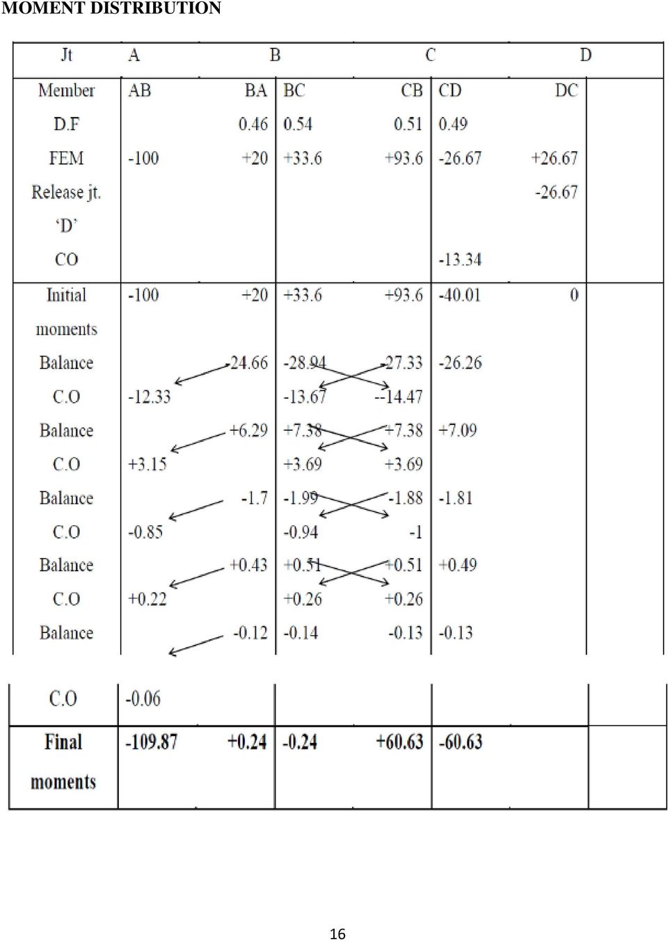
16 MOMENT DISTRIBUTION 16

17 BMD MOMENT DISTRIBUTION FOR FRAMES WITH NO SIDE SWAY The analysis of such a frame when the loading conditions and the geometry of the frame is such that there is no joint translation or sway, is similar to that given for beams. 3. Q. Analysis the frame shown in figure by moment distribution method and draw BMD assume EI is constant. 17

18 DISTRIBUTION FACTOR 18

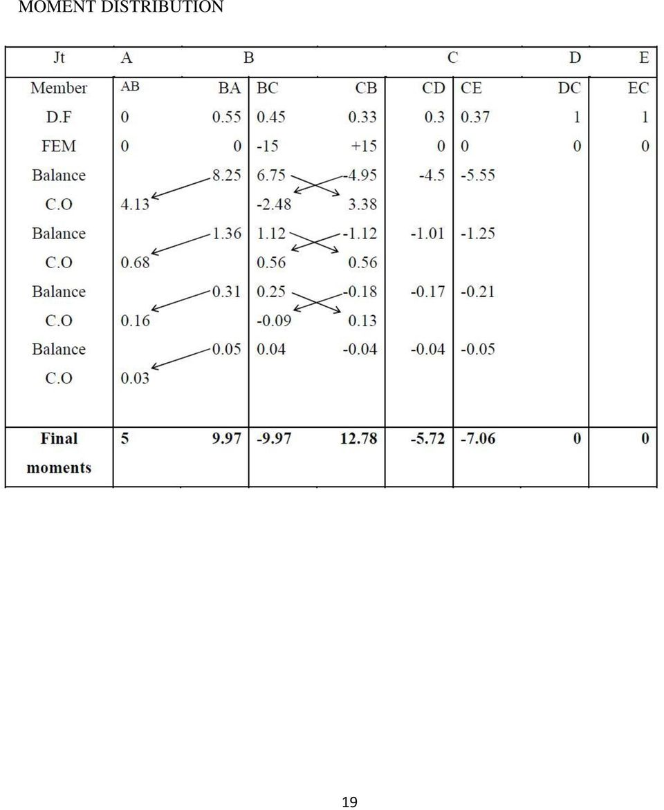
19 MOMENT DISTRIBUTION 19

20 MOMENT DISTRIBUTION METHOD FOR FRAMES WITH SIDE SWAY Frames that are non symmetrical with reference to material property or geometry (different lengths and I values of column) or support condition or subjected to non-symmetrical loading have a tendency to side sway. 4.Q. Analyze the frame shown in figure by moment distribution method. Assume EI is constant. 20

21 A. Non Sway Analysis: First consider the frame without side sway 21

22 DISTRIBUTION FACTOR DISTRIBUTION OF MOMENTS FOR NON-SWAY ANALYSIS 22

23 FREE BODY DIAGRAM OF COLUMNS By seeing of the FBD of columns R = (Using F x =0 for entire frame) = 0.91 KN Now apply R = 0.91 KN acting opposite as shown in the above figure for the sway analysis. Sway analysis: For this we will assume a force R is applied at C causing the frame to deflect as shown in the following figure. 23

24 Since both ends are fixed, columns are of same length & I and assuming joints B & C are temporarily restrained from rotating and resulting fixed end moment are Assume 24

25 Moment distribution table for sway analysis: Free body diagram of columns Using F x = 0 for the entire frame R = = 56 KN 25

26 Hence R = 56KN creates the sway moments shown in above moment distribution table. Corresponding moments caused by R = 0.91KN can be determined by proportion. Thus final moments are calculated by adding non sway moments and sway. Moments calculated for R = 0.91KN, as shown below. BMD 26

27 5.Q. Analysis the rigid frame shown in figure by moment distribution method and draw BMD A. Non Sway Analysis: First consider the frame held from side sway 27

28 DISTRIBUTION FACTOR DISTRIBUTION OF MOMENTS FOR NON-SWAY ANALYSIS 28

29 FREE BODY DIAGRAM OF COLUMNS Applying Fx = 0 for frame as a Whole, R = = 5.34 KN Now apply R = 5.34KN acting opposite Sway analysis: For this we will assume a force R is applied at C causing the frame todeflect as shown in figure 29

30 Assume MOMENT DISTRIBUTION FOR SWAY ANALYSIS FREE BODY DIAGRAMS OF COLUMNS AB &CD 30

31 16.36 KNm KN KNm 8.78 KN 2.34 KN Using Fx = 0 for the entire frame R = kn Hence R = KN creates the sway moments shown in the above moment distribution table. Corresponding moments caused by R = 5.34 kn can be determined by proportion. Thus final moments are calculated by adding non-sway moments and sway moments determined for R = 5.34 KN as shown below. 20 KNm 31

32 19.78 KNm 4.63KNm 4.63KN m KNm 17.4KNm B.M.D 32

33 PART B : KANI S METHOD OF ANALYSIS This method was developed by Dr. Gasper Kani of Germany in This method offers an iterative scheme for applying slope deflection method. We shall now see the application of Kani s method for different cases. BEAMS WITH NO TRANSLATION OF JOINTS: 33

34 Let AB represent a beam in a frame, or a continuous structure under transverse loading, as show in fig. 1 (a) let the M AB & M BA be the end moment at ends A & B respectively. Sign convention used will be: clockwise moment +ve and anticlockwise moment ve. The end moments in member AB may be thought of as moments developed due to a superposition of the following three components of deformation. 1. The member AB is regarded as completely fixed. (Fig. 1 b). The fixed end moments for this condition are written as M FAB & M FBA, at ends A & B respectively. 2. The end A only is rotated through an angle A by a moment 2 M ' AB inducing a moment M ' AB at fixed end B. 3. Next rotating the end B only through an angle B by moment 2M ' BA while keeping end A as fixed. This induces a moment M ' BAat end A. Thus the final moment MAB & MBA can be expressed as super position of three moments For member AB we refer end A as near end and end B as far end. Similarly when we refer to moment M BA, B is referred as near end and end A as far end. Hence above equations can be stated as follows. The moment at the near end of a member is the algebraic sum of (a) fixed end moment at near end. (b) Twice the rotation moment of the near end (c) rotation moment of the far end. Rotation factors: Fig. 2 shows a multistoried frame. 34

35 Consider various members meeting at joint A. If no translations of joints occur, applying equation (1), for the end moments at A for the various members meeting at A are given by: M AB = M FAB + 2M ' AB M AC = M FAC + 2M ' AC + M ' BA + M CA ' M AD = M FAD + 2 M ' AD M AE = M FAE + 2M ' AE + M ' DA + M ' EA 35

36 Analysis Method: In equation (6) M FAB is a known quantity. To start with the far end rotation moments M ' BA are not known and hence they may be taken as zero. By a similar approximation the rotation moments at other joints are also determined. With the approximate values of rotation moments computed, it is possible to again determine a more correct value of the rotation moment at A from member AB using equation (6). The process is carried out for sufficient number of cycles until the desired degree of accuracy is achieved. 36

37 The final end moments are calculated using equation (1). Kani s method for beams without translation of joints, is illustrated in followingexamples: Ex: 1 Analyze the beam show in fig 3 (a) by Kani s method and draw bending moment diagram Solution: a) Fixed end moments: b) Rotation Factors: 37

38 1 Jt. Member Relative K Rotation Factor stiffness (K) B BA I/5 = 0.2I BC 2I/4 = 0.5I 0.7I C CB 2I/4 = 0.5I CD I/5 = 0.2I 0.7I c) Sum fixed end moment at joints: The scheme for proceeding with method of rotation contribution is shown in figure 3 (b). The FEM, rotation factors and sum of fixed end moments are entered in appropriate places as shown in figure 3 (b). 38

39 d) Iteration Process: Rotation contribution values at fixed ends A &D are zero. Rotation contributions at joints B & C are initially assumed as zero arbitrarily. These values will be improved in iteration cycles until desired degree of accuracy is achieved. The calculations for two iteration cycles have been shown in following table. The remaining iteration cycle values for rotation contributions along with these two have been shown directly in figure 3 (c). Iterations are done up to four cycles yielding practically the same value of rotation contributions. d) Final moments: Bending moment diagram is shown in fig.3 (d) 39

40 Fig.3 (d) Ex 2: Analyze the continuous beam shown in fig. 4 (a) Solution: a) Fixed end moments: 40

41 b) Modification in fixed end moments: Actually end D is a simply supported. Hence moment at D should be zero. To make moment at D as zero apply 8 knm at D and perform the corresponding carry over to CD. 41

42 42

43 Iteration process has been stopped after 4 th cycle since rotation contribution values are becoming almost constant. Values of fixed end moments, sum of fixed end moments, rotation factors along with rotation contribution values after end of each cycle in appropriate places has been shown in fig. 4 (b). BMD is shown below: 43

44 Ex 3: Analyze the continuous beam shown in fig. 5 (a) and draw BMD & SFD (VTU January 2005 exam) Solution: a) Fixed end moments: b) Modification in fixed end moments: Since M CD = - 5 knm; M CB = + 5kNm, for this add 1.25 knm to M FCB and do the corresponding carry over to M FBC Now M CB = 5 knm 44

45 Now joint C will not enter in the iteration process. c) Rotation factors: Relative stiffness Rotation Factor Jt. Member (K) B BA I/4 = 0.25I -0.2 BC 3 1.5I = I 0.625I C CB 1.5I/3 = 0.5I CD 0 0.5I 0 d) Sum of fixed end moments at joints: M FB = = 3.54 knm e) Iteration Process 45

46 Since B is the only joint needing rotation correction, the iteration process will stop after first iteration. Value of FEMs, sum of FEM at joint, rotation factors along with rotation contribution values in appropriate places is shown in fig. 5 (b) Fig.5(b) 46

47 (f) Final moments: FBD of each span along with reaction values which have been calculated from statics are shown below: BMD and SFD are shown below 47

48 KANI S METHOD FOR MEMBERS WITH TRANSLATORY JOINTS Fig. 6 shows a member AB in a frame which has undergone lateral displacement at A & B so that the relative displacement is If ends A & B are restrained from rotation FEM corresponding to this displacement are When translation of joints occurs along with rotations the true end moments are given by M AB = M FAB + 2M ' AB + M ' BA + M ' AB ' 48

49 M BA = M FBA + 2M ' BA + M ' AB + M ' BA ' If A happens to be a joint where two or more members meet then from equilibrium of joint we have Using the above relationships rotation contributions can be determined by iterative procedure. If lateral displacements are known the displacement moments can be determined from equation (7). If lateral displacements are unknown then additional equations have to be developed for analyzing the member. Ex 4: In a continuous beam shown in fig. 7 (a). The support B sinks by 10mm. Determine the moments by Kani s method & draw BMD. 49

50 Solution: (a) Calculation of FEM: 50

51 b) Modification in fixed end moments: Since end D is a simply supported, moment at D is zero. To make moment at D as zero apply a moment of over to CD knm at end D and perform the corresponding carry Other FEMs will be same as calculated earlier. Now joint D will not enter the iteration process. c) Rotation factors: 51

52 Relative stiffness Rotation Factor 1 K Joint Member K (K) U = - x 2 K B BA I/6 = 0.17 I I BC I/5 = 0.2 I C CB I/5 = 0.2I CD 3 x I/4 = 0.19 I I d) Sum of fixed end moments: e) Iteration process: 52

53 Iteration process has been stopped after fourth cycle since rotation contribution values are becoming almost constant. Values of FEMs, sum of fixed end moments, rotation factors along with rotation contribution values after end of each cycle in appropriate places has been shown in Fig. 7 (b). 53

54 g) BMD is shown below: x3x2/5 = 60 20x6² / 8 = 90 20x4²/8 = 40KNM KNM KNM 54

55 ANALYSIS OF FRAMES WITH NO TRANSLATION OF JOINTS The frames, in which lateral translations are prevented, are analyzed in the same way as continuous beams. The lateral sway is prevented either due to symmetry of frame and loading or due to support conditions. The procedure is illustrated in following example. Example-5. Analyze the frame shown in Figure 8 (a) by Kani s method. Draw BMD. Fig-8(a) Solution: (a) Fixed end moments: 55

56 (b) Rotation factors: Joint Member Relative Stiffness (k) k Rotation factor = -½k/ k B BC 3I/6 = 0.5I 0.83I -0.3 BA I/3 = 0.33I -0.2 C CB 3I/6 = 0.5I 0.83I -0.3 CD I/3 = 0.33I

57 (c) Sum of FEM: (d) Iteration process: Joint B C Rotation M BA M BC M CB M CD Contribution Rotation Factor Iteration 1-0.2(-120+0) -0.3(-120+0) -0.2( ) -0.2( ) Stated with =24 =36 = = end B taking M AB =0 and assuming M CB =0 Iteration 2-0.2( ) -0.3( ) -0.3( ) -0.2( ) =33.6 =50.04 = = Iteration 3-0.2( ) -0.3( ) -0.3( ) -0.2 ( ) =34.2 =51.3 = = Iteration 4-0.2( ) -0.3( ) -0.3( ) -0.2 ( ) =34.28 =51.42 = =

58 The fixed end moments, sum of fixed and moments, rotation factors along with rotation contribution values at the end of each cycle in appropriate places is shown in figure 8(b). Fig-8(b) 58

59 (e) Final moments: Member MFij 2M ij (knm) M ji (knm) (ij) (knm) Final moment = M Fij + 2M ij + M ji AB BA 0 2 x BC x CB x (-51.43) CD 0 2 x (-34.28) DC BMD is shown below in figure-8 (c) 59

60 Fig-8 (c) 60

61 ANALYSIS OF SYMMETRICAL FRAMES UNDER SYMMETRICAL LOADING Considerable calculation work can be saved if we make use of symmetry of frames and loading especially when analysis is done manually. Two cases of symmetry arise, namely, frames in which the axis of symmetry passes through the centerline of the beams and frames with the axis of symmetry passing through column line. Case-1: (Axis of symmetry passes through center of beams): Let AB be a horizontal member of the frame through whose center, axis of symmetry passes. Let M ab and M ba be the end moments. Due to symmetry of deformation M ab and M ba are numerically equal but are opposite in their sense. Let this member be replaced by member AB whose end A will undergo the rotation A due to moment M ab applied at A, the end B being fixed. 61

62 Hence for equality of rotations between original member AB and the substitute member AB Thus if K is the relative stiffness of original member AB, this member can be replaced by substitute member AB having relative stiffness K. With this substitute2 member, the analysis need to be carried out for only, one half of the frame considering line of symmetry as fixed. 62

63 Example-6: Analyze the frame given in example-5 by using symmetry condition by Kani s method. Solution: Since symmetry axis passes through center of beam only one half of frame as shown in figure 9 (a) will be considered Fig-9(a) U BA = U BC = The calculation of rotation contribution values is shown directly in figure-9(b) 63

64 Fig-9(b) 64

65 Here we can see that rotation contributions are obtained in the first iteration only. The final moments for half the frame are shown in figure 9(c) and for full frame are shown in figure 9(d). Fig-9(c) Fig-9(d) 65

66 Example-7: Analyze the frame shown in figure 10(a) by Kani s method. Fig-10(a) Solution: Analysis will be carried out taking the advantage of symmetry (a) Fixed end moments: 66

67 The substitute frame is shown in figure 10(b) D KCD = 1 2 x2 4 I =4 I Fig-10(b) Kba = 2I = I 4 2 (b) Rotation factors: 1 K Joint Member Relative Stiffness K k Rotation factors = 2 ΣK B BA 2I/4 5I/4-1/5 BE 1x 4I =I / 2-1/5 2 4 BC I/ C CB I/4 2I/4-1/4 CD 1x 2I= I -1/ Rotation contributions calculated by iteration process are directly shown in figure- 10(c). 67

68 ' Fig-10(c) ' 68

69 The calculation of final moments for the substitute frame is shown in figure- 10(d) Fig-10(d) 69

70 Figure-10(e) shows final end moments for the entire frame. Fig-10(e) 70

71 Case 2: When the axis of symmetry passes through the column: This case occurs when the number of bays is an even number. Due to symmetry of the loading and frame, the joints on the axis of symmetry will not rotate. Hence it is sufficient if half the frame is analyzed. The following example illustrates the procedure. Example-8: Analyze the frame shown in figure-11(a) by Kani s method, taking advantage of symmetry and loading. Solution: Fig-11(a) Only half frame as shown in figure-11(b) will be considered for the analysis. D Fig-11(b) 71

72 The iteration process for calculation of rotation contribution values at C & B was carried up to four cycles and values for each cycle are shown in figure-11(c). Fig-11(c) 72

73 Final moments calculations for half the frame are shown in figure-11(d) and final end moments of all the members of the frame are shown in figure-11(e). E Fig-11(d) 73

74 74

75 UNIT II: ANALYSIS OF FRAMES AND ARCHES PART A: THE SLOPE DEFLECTION METHOD In the slope-deflection method, the relationship is established between moments at the ends of the members and the corresponding rotations and displacements. The slope-deflection method can be used to analyze statically determinate and indeterminate beams and frames. In this method it is assumed that all deformations are due to bending only. In other words deformations due to axial forces are neglected. In the force method of analysis compatibility equations are written in terms of unknown reactions. It must be noted that all the unknown reactions appear in each of the compatibility equations making it difficult to solve resulting equations. The slopedeflection equations are not that lengthy in comparison. The basic idea of the slope deflection method is to write the equilibrium equations for each node in terms of the deflections and rotations. Solve for the generalized displacements. Using momentdisplacement relations, moments are then known. The structure is thus reduced to a determinate structure. The slope-deflection method was originally developed by Heinrich Manderla and Otto Mohr for computing secondary stresses in trusses. The method as used today was presented by G.A.Maney in 1915 for analyzing rigid jointed structures. FUNDAMENTAL SLOPE-DEFLECTION EQUATIONS: The slope deflection method is so named as it relates the unknown slopes and deflections to the applied load on a structure. In order to develop general form of slope deflection equations, we will consider the typical span AB of a continuous beam which is subjected to arbitrary loading and has a constant EI. We wish to relate the beams internal end moments in terms of its three degrees of freedom, namely its angular displacements and linear displacement which could be caused by relative settlements between the supports. Since we will be developing a formula, moments and angular displacements will be considered positive, when they act clockwise on the span. The linear displacement will be considered positive since this displacement causes the chord of the span and the span s chord angle to rotate clockwise. The slope deflection equations can be obtained by using principle of superposition by considering separately the moments developed at each supports due to each of the displacements and then the load. 75

76 Case A: fixed-end moments 76

77 Case B: rotation at A, (angular displacement at A) Consider node A of the member as shown in figure to rotate while its far end B is fixed. To determine the moment needed to cause the displacement, we will use conjugate beam method. The end shear at A` acts downwards on the beam since is clockwise. Case C: rotation at B, (angular displacement at B) In a similar manner if the end B of the beam rotates to its final position, while end A is held fixed. We can relate the applied moment to the angular displacement and the reaction moment Case D: displacement of end B related to end A If the far node B of the member is displaced relative to A so that so that the chord of the member rotates clockwise (positive displacement).the moment M can be related to displacement by using conjugate beam method. The conjugate beam is free at both the ends as the real beam is fixed supported. Due to displacement of the real beam at B, the moment at 77

78 the end B` of the conjugate beam must have a magnitude of.summing moments about B` we have, By our sign convention the induced moment is negative, since for equilibrium it acts counter clockwise on the member. If the end moments due to the loadings and each displacements are added together, then the resultant moments at the ends can be written as, 78

79 FIXED END MOMENT TABLE 79

80 80

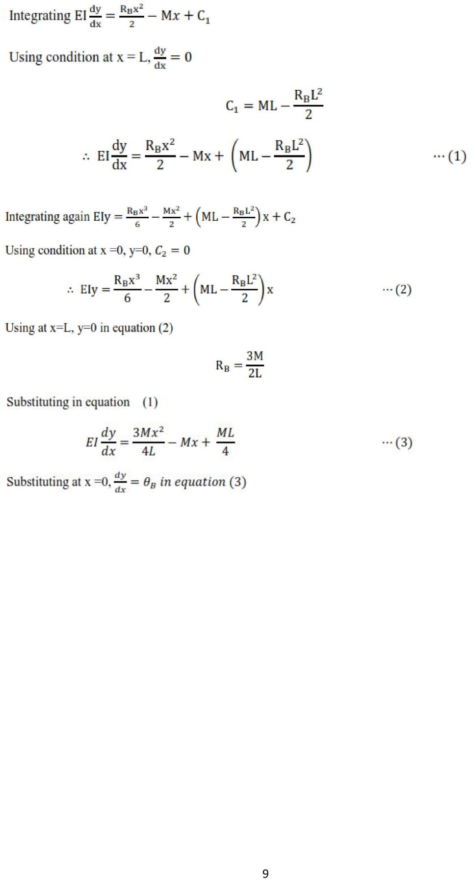
81 GENERAL PROCEDURE OF SLOPE-DEFLECTION METHOD Find the fixed end moments of each span (both ends left & right). Apply the slope deflection equation on each span & identify the unknowns. Write down the joint equilibrium equations. Solve the equilibrium equations to get the unknown rotation & deflections. Determine the end moments and then treat each span as simply supported beam subjected to given load & end moments so we can work out the reactions & draw the bending moment & shear force diagram. Numerical Examples 1. Q. Analyze two span continuous beam ABC by slope deflection method. Then draw Bending moment & Shear force diagram. Take EI constant. Fixed end moments are 81

82 Slope deflection equations are In all the above 4 equations there are only 2 unknowns boundary and accordingly the conditions are Solving the equations (5) & (6), we get Substituting the values in the slope deflections we have, Reactions: Consider the free body diagram of the beam 82

83 Find reactions using equations of equilibrium. Span AB: M A = 0, R B 6 = R B = KN V = 0, R A +R B = 100KN R A = =29.40 KN Span BC: M C = 0, R B 5 = R B = 65 KN V=0 R B +R C = 20 5 = 100KN R C = = 35 KN Using these data BM and SF diagram can be drawn 83

84 Max BM: Span AB: Max BM in span AB occurs under point load and can be found geometrically, Span BC: Max BM in span BC occurs where shear force is zero or changes its sign. Henceconsider SF equation w.r.t C Max BM occurs at 1.75m from 84

85 2. Q. Analyze continuous beam ABCD by slope deflection method and then draw bending moment diagram. Take EI constant. Slope deflection equations are In all the above equations there are only 2 unknowns and accordingly the boundary conditions are 85

86 Solving equations (5) & (6), Substituting the values in the slope deflections we have, Reactions: Consider free body diagram of beam AB, BC and CD as shown 86

87 Span AB: 87

88 Maximum Bending Moments: Span AB: Occurs under point load Span BC: Where SF=0, consider SF equation with C as reference 3. Q. Analyse the continuous beam ABCD shown in figure by slope deflection method. The support B sinks by 15mm.Take E = KN/m 2 and I = m 4 FEM due to yield of support B 88

89 For span AB: For span BC: Slope deflection equations are In all the above equations there are only 2 unknowns boundary and accordingly the conditions are 89

90 Solving equations (5) & (6), Substituting the values in the slope deflections we have, Consider the free body diagram of continuous beam for finding reactions REACTIONS Span AB: 90

91 91

92 ANALYSIS OF FRAMES (WITHOUT & WITH SWAY) The side movement of the end of a column in a frame is called sway. Sway can be prevented by unyielding supports provided at the beam level as well as geometric or load symmetry about vertical axis. Frame with sway Sway prevented by unyielding support 92

93 4. Q. Analyse the simple frame shown in figure. End A is fixed and ends B & C are hinged. Draw the bending moment diagram. Slope deflection equations are 93

94 In all the above equations there are only 3 unknowns and accordingly the boundary conditions are Solving equations (7) & (8) & (9), Substituting the values in the slope deflections we have, 94

95 REACTIONS: SPAN AB: SPAN BC: Column BD: 95

96 5.Q. Analyse the portal frame and then draw the bending moment diagram A. This is a symmetrical frame and unsymmetrically loaded, thus it is an unsymmetrical problem and there is a sway,assume sway to right 96

97 FEMS: Slope deflection equations are 97

98 98

99 Reactions: consider the free body diagram of beam and columns Column AB: Span BC: Column CD: 99

100 Check: Hence okay 6. Q. Frame ABCD is subjected to a horizontal force of 20 KN at joint C as shown in figure. Analyse and draw bending moment diagram. 100

101 A. The frame is symmetrical but loading is unsymmetrical. Hence there is a sway, assume sway towards right. In this problem FEMS Slope deflection equations: 101

102 102

103 103

104 Reactions: Consider the free body diagram of various members Member AB: Span BC: Column CD: Check: 104

105 7.Q.Analyse the portal frame and draw the B.M.D. A. It is an unsymmetrical problem, hence there is a sway be towards right. FEMS: Slope deflection equations: 105

106 106

107 107

108 Reactions: Consider the free body diagram Member AB: Span BC: Column CD: Check: 108

109 109

110 PART B : TWO HINGED ARCHES INTRODUCTION Mainly three types of arches are used in practice: three-hinged, two-hinged and hingeless arches. In the early part of the nineteenth century, three-hinged arches were commonly used for the long span structures as the analysis of such arches could be done with confidence. However, with the development in structural analysis, for long span structures starting from late nineteenth century engineers adopted two-hinged and hingeless arches. Two-hinged arch is the statically indeterminate structure to degree one. Usually, the horizontal reaction is treated as the redundant and is evaluated by the method of least work. In this lesson, the analysis of two-hinged arches is discussed and few problems are solved to illustrate the procedure for calculating the internal forces. ANALYSIS OF TWO-HINGED ARCH A typical two-hinged arch is shown in Fig. 33.1a. In the case of two-hinged arch, we have four unknown reactions, but there are only three equations of equilibrium available. Hence, the degree of statical indeterminacy is one for twohinged arch. 110

111 The fourth equation is written considering deformation of the arch. The unknown redundant reaction H b is calculated by noting that the horizontal displacement of hinge B is zero. In general the horizontal reaction in the two hinged arch is evaluated by straightforward application of the theorem of least work (see module 1, lesson 4), which states that the partial derivative of the strain energy of a statically indeterminate structure with respect to statically indeterminate action should vanish. Hence to obtain, horizontal reaction, one must develop an expression for strain energy. Typically, any section of the arch (vide Fig 33.1b) is subjected to shear forcev, bending moment M and the axial compression N. The strain energy due to bending U b is calculated from the following expression. 111

112 The above expression is similar to the one used in the case of straight beams. However, in this case, the integration needs to be evaluated along the curved arch length. In the above equation, s is the length of the centerline of the arch, I is the moment of inertia of the arch cross section, E is the Young s modulus of the arch material. The strain energy due to shear is small as compared to the strain energy due to bending and is usually neglected in the analysis. In the case of flat arches, the strain energy due to axial compression can be appreciable and is given by, The total strain energy of the arch is given by 112

113 113

114 114

115 TEMPERATURE EFFECT Consider an unloaded two-hinged arch of span L. When the arch undergoes a uniform temperature change of T, then its span would increase by C TLα if it were allowed to expand freely (vide Fig 33.3a). α is the co-efficient of thermal expansion of the arch material. Since the arch is restrained from the horizontal movement, a horizontal force is induced at the support as the temperature is increase Now applying the Castigliano s first theorem, Solving for H, The second term in the denominator may be neglected, as the axial rigidity is quite high. Neglecting the axial rigidity, the above equation can be written as 115

116 Example A semicircular two hinged arch of constant cross section is subjected to a concentrated load as shown in Fig. Calculate reactions of the arch and draw bending moment diagram. Solution: Taking moment of all forces about hinge B leads to, 116

117 From figure, 117

118 Bending moment diagram Bending moment M at any cross section of the arch is given by, 118

119 Using equations (8) and (9), bending moment at any angle θ can be computed. The bending moment diagram is shown in Fig. Example A two hinged parabolic arch of constant cross section has a span of 60m and a rise of 10m. It is subjected to loading as shown in Fig.. Calculate reactions of the arch if the temperature of the arch is raised by. Assume co-efficient of thermal expansion as 119

120 Taking A as the origin, the equation of two hinged parabolic arch may be written as, The given problem is solved in two steps. In the first step calculate the horizontal reaction due to 40kN load applied at C. In the next step calculate the horizontal reaction due to rise in temperature. Adding both, one gets the horizontal reaction at the hinges due to 40kN combined external loading and temperature change. The horizontal reaction due to load may be calculated by the following equation, Please note that in the above equation, the integrations are carried out along the x- axis instead of the curved arch axis. The error introduced by this change in the variables in the case of flat arches is negligible. Using equation (1), the above equation (3) can be easily evaluated. The vertical reaction A is calculated by taking moment of all forces about B. Hence, 120

121 121

122 Table 1. Numerical integration of equations (8) and (9) 122

123 Summary Two-hinged arch is the statically indeterminate structure to degree one. Usually, the horizontal reaction is treated as the redundant and is evaluated by the method of least work. Towards this end, the strain energy stored in the two-hinged arch during deformation is given. The reactions developed due to thermal loadings are discussed. Finally, a few numerical examples are solved to illustrate the procedure. 123

124 UNIT III: APPROXIMATE METHODS OF ANALYSIS OF BUILDING FRAMES INTRODUCTION The building frames are the most common structural form, an analyst/engineer encounters in practice. Usually the building frames are designed such that the beam column joints are rigid. A typical example of building frame is the reinforced concrete multistory frames. A two-bay, three-storey building plan and sectional elevation are shown in Fig.. In principle this is a three dimensional frame. However, analysis may be carried out by considering planar frame in two perpendicular directions separately for both vertical and horizontal loads as shown in Fig and finally superimposing moments appropriately. In the case of building frames, the beam column joints are monolithic and can resist bending moment, shear force and axial force. The frame has 12 joints j, 15 beam members b, and 9 reaction components r. Thus this frame is statically indeterminate to degree 3x 15912x318 (Please see lesson 1, module 1for more details). Any exact method, such as slope-deflection method, moment distribution method or direct stiffness method may be used to analyse this rigid frame. However, in order to estimate the preliminary size of different members, approximate methods are used to obtain approximate design values of moments, shear and axial forces in various members. Before applying approximate methods, it is necessary to reduce the given indeterminate structure to a determinate structure by suitable assumptions. These will be discussed in this lesson. In next section, analysis of building frames to vertical loads is discussed and in section after that, analysis of building frame to horizontal loads will be discussed. 124

125 125

126 126

127 SUBSTITUTE FRAME METHOD Consider a building frame subjected to vertical loads as shown in Fig Any typical beam, in this building frame is subjected to axial force, bending moment and shear force. Hence each beam is statically indeterminate to third degree and hence 3 assumptions are required to reduce this beam to determinate beam. Before we discuss the required three assumptions consider a simply supported beam. In this case zero moment (or point of inflexion) occurs at the supports as shown in Fig.36.4a. Next consider a fixed-fixed beam, subjected to vertical loads as shown in Fig. 36.4b. In this case, the point of inflexion or point of zero moment occurs at 0.21L from both ends of the support. 127

128 Now consider a typical beam of a building frame as shown in Fig.36.4c. In this case, the support provided by the columns is neither fixed nor simply supported. For the purpose of approximate analysis the inflexion point or point of zero the point of zero moment varies depending on the actual rigidity provided by the columns. Thus the beam is approximated for the analysis as shown in Fig. 128

129 129

130 For interior beams, the point of inflexion will be slightly more than 0.1L. An experienced engineer will use his past experience to place the points of inflexion appropriately. Now redundancy has reduced by two for each beam. The third assumption is that axial force in the beams is zero. With these three assumptions one could analyse this frame for vertical loads. Example 36.1 Analyse the building frame shown in Fig. 36.5a for vertical loads using approximate methods. 130

131 Solution: In this case the inflexion points are assumed to occur in the beam at 0.1L0.6m from columns as shown in Fig. 36.5b. The calculation of beam moments is shown in Fig. 36.5c. 131

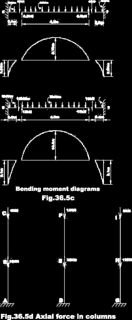
132 132

133 Now the beam ve moment is divided equally between lower column and upper column. It is observed that the middle column is not subjected to any moment, as the moment from the right and the moment from the left column balance each other. The ve moment in the beam BE is 8.1kN.m. Hence this moment is divided between column BC andba. Hence,M BC M BA kN.m. The maximum ve moment in beam BE is 14.4 kn.m. The columns do carry axial loads. The axial compressive loads in the columns can be easily computed. This is shown in Fig. 36.5d. ANALYSIS OF BUILDING FRAMES TO LATERAL (HORIZONTAL) LOADS A building frame may be subjected to wind and earthquake loads during its life time. Thus, the building frames must be designed to withstand lateral loads. A two-storey two-bay multistory frame subjected to lateral loads is shown in Fig The actual deflected shape (as obtained by exact methods) of the frame is also shown in the figure by dotted lines. The given frame is statically indeterminate to degree

134 134

135 Hence it is required to make 12 assumptions to reduce the frame in to a statically determinate structure. From the deformed shape of the frame, it is observed that inflexion point (point of zero moment) occur at mid height of each column and mid point of each beam. This leads to 10 assumptions. Depending upon how the remaining two assumptions are made, we have two different methods of analysis: i) Portal method and ii) cantilever method. They will be discussed in the subsequent sections. PORTAL METHOD In this method following assumptions are made. 1) An inflexion point occurs at the mid height of each column. 2) An inflexion point occurs at the mid point of each girder. 135

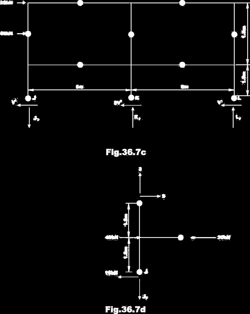
136 3) The total horizontal shear at each storey is divided between the columns of that storey such that the interior column carries twice the shear of exterior column. The last assumption is clear, if we assume that each bay is made up of a portal thus the interior column is composed of two columns (Fig. 36.6). Thus the interior column carries twice the shear of exterior column. This method is illustrated in example Example 36.2 Analyse the frame shown in Fig. 36.7a and evaluate approximately the column end moments, beam end moments and reactions. Solution: The problem is solved by equations of statics with the help of assumptions made in the portal method. In this method we have hinges/inflexion points at mid height of columns and beams. Taking the section through column hinges M.N,O we get, (ref. Fig. 36.7b). 136

137 137

138 138

139 139

140 Column and beam moments are calculated as, (ref. Fig. 36.7f) M BC 5x kn.m ; M BA 15x kn.m M BE 30 kn.m M EF 10x1.515 kn.m ; M ED 30x1.545 kn.m M EB 30 kn.m M EH 30 kn.m M HI 5x kn.m ; M HG 15x kn.m M HE 30 kn.m Reactions at the base of the column are shown in Fig. 36.7g. 140

141 CANTILEVER METHOD The cantilever method is suitable if the frame is tall and slender. In the cantilever method following assumptions are made. 1) An inflexion point occurs at the mid point of each girder. 2) An inflexion point occurs at mid height of each column. 3) In a storey, the intensity of axial stress in a column is proportional to its horizontal distance from the center of gravity of all the columns in that storey. Consider a cantilever beam acted by a horizontal load P as shown in Fig In such a column the bending stress in the column cross section varies linearly from its neutral axis. The last assumption in the cantilever method is based on this fact. The method is illustrated in example Example 36.3 Estimate approximate column reactions, beam and column moments using cantilever method of the frame shown in Fig. 36.8a. The columns are assumed to have equal cross sectional areas. Solution: This problem is already solved by portal method. The center of gravity of all column passes through centre column. B. xa 0 A5A10A 5 m (from left column) AA A A 141

142 142

143 Taking a section through first storey hinges gives us the free body diagram as shown in Fig. 36.8b. Now the column left of C.G. i.e.cb must be subjected to tension and one on the right is subjected to compression. From the third assumption, Taking moment about O of all forces gives, Taking moment about R of all forces left of R, 143

144 Taking moment of all forces right of S about S, Moments M CB kn.m M CF 7.5 kn.m M FE 15 kn.m M FC 7.5 kn.m M FI 7.5 kn.m M IH 7.5 kn.m M IF 7.5 kn.m Tae a section through hinges J,K,L (ref. Fig. 36.8c). Since the center of gravity passes through centre column the axial force in that column is zero. 144

145 Taking moment about hinge L, J y can be evaluated. Thus, Taking moment of all forces left of P about P gives, Similarly taking moment of all forces right of Q about Q gives, 145

146 Moments M BC kn.m ; M BA kn.m M BE 30 kn.m M EF kn.m ; M ED kn.m M EB 30 kn.m M EH 30 kn.m M HI kn.m ; M HG kn.m M HE 30 kn.m In this lesson, the building frames are analysed by approximate methods. Towards this end, the given indeterminate building fame is reduced into a determinate structure by suitable assumptions. The analysis of building frames to vertical loads was discussed in section In section 36.3, analysis of building frame to horizontal loads is discussed. Two different methods are used to analyse building frames to horizontal loads: portal and cantilever method. Typical numerical problems are solved to illustrate the procedure. 146

147 PART B Approximate Lateral Load Analysis by Portal Method Portal Frame Portal frames, used in several Civil Engineering structures like buildings, factories, bridges have the primary purpose of transferring horizontal loads applied at their tops to their foundations. Structural requirements usually necessitate the use of statically indeterminate layout for portal frames, and approximate solutions are often used in their analyses. Assumptions for the Approximate Solution In order to analyze a structure using the equations of statics only, the number of independent force components must be equal to the number of independent equations of statics. If there are n more independent force components in the structure than there are independent equations of statics, the structure is statically indeterminate to the nth degree. Therefore to obtain an approximate solution of the structure based on statics only, it will be necessary to make n additional independent assumptions. A solution based on statics will not be possible by making fewer than n assumptions, while more than n assumptions will not in general be consistent. Thus, the first step in the approximate analysis of structures is to find its degree of statical indeterminacy (dosi) and then to make appropriate number of assumptions. For example, the dosi of portal frames shown in (i), (ii), (iii) and (iv) are 1, 3, 2 and 1 respectively. Based on the type of frame, the following assumptions can be made for portal structures with a vertical axis of symmetry that are loaded horizontally at the top 1. The horizontal support reactions are equal 2. There is a point of inflection at the center of the unsupported height of each fixed based column Assumption 1 is used if dosi is an odd number (i.e., = 1 or 3) and Assumption 2 is used if dosi

148 Some additional assumptions can be made in order to solve the structure approximately for different loading and support conditions. 3. Horizontal body forces not applied at the top of a column can be divided into two forces (i.e., applied at the top and bottom of the column) based on simple supports 4. For hinged and fixed supports, the horizontal reactions for fixed supports can be assumed to be four times the horizontal reactions for hinged supports Example Draw the axial force, shear force and bending moment diagrams of the frames loaded as shown below. 148

149 149

150 Analysis of Multi-storied Structures by Portal Method Approximate methods of analyzing multi-storied structures are important because such structures are statically highly indeterminate. The number of assumptions that must be made to permit an analysis by statics alone is equal to the degree of statical indeterminacy of the structure. Assumptions The assumptions used in the approximate analysis of portal frames can be extended for the lateral load analysis of multi-storied structures. The Portal Method thus formulated is based on three assumptions 1. The shear force in an interior column is twice the shear force in an exterior column. 2. There is a point of inflection at the center of each column. 3. There is a point of inflection at the center of each beam. Assumption 1 is based on assuming the interior columns to be formed by columns of two adjacent bays or portals. Assumption 2 and 3 are based on observing the deflected shape of the structure. Example Use the Portal Method to draw the axial force, shear force and bending moment diagrams of the three-storied frame structure loaded as shown below. 150

151 Analysis of Multi-storied Structures by Cantilever Method Although the results using the Portal Method are reasonable in most cases, the method suffers due to the lack of consideration given to the variation of structural response due to the difference between sectional properties of various members. The Cantilever Method attempts to rectify this limitation by considering the crosssectional areas of columns in distributing the axial forces in various columns of a story. Assumptions The Cantilever Method is based on three assumptions 1. The axial force in each column of a storey is proportional to its horizontal distance from the centroidal axis of all the columns of the storey. 2. There is a point of inflection at the center of each column. 3. There is a point of inflection at the center of each beam. Assumption 1 is based on assuming that the axial stresses can be obtained by a method analogous to that used for determining the distribution of normal stresses 151

152 on a transverse section of a cantilever beam. Assumption 2 and 3 are based on observing the deflected shape of the structure. Example Use the Cantilever Method to draw the axial force, shear force and bending moment diagrams of the three -storied frame structure loaded as shown below. Approximate Vertical Load Analysis Approximation based on the Location of Hinges If a beam AB is subjected to a uniformly distributed vertical load of w per unit length [Fig. (a)], both the joints A and B will rotate as shown in Fig. (b), because although the joints A and B are partly restrained against rotation, the restraint is not complete. Had the joints A and B been completely fixed against rotation [Fig. (c)] the points of inflection 152

153 would be located at a distance 0.21L from each end. If, on the other hand, the joints A and B are hinged [Fig. (d)], the points of zero moment would be at the end of the beam. For the actual case of partial fixity, the points of inflection can be assumed to be somewhere between 0.21 L and 0 from the end of the beam. For approximate analysis, they are often assumed to be located at one-tenth (0.1 L) of the span length from each end joint. Depending on the support conditions (i.e., hinge ended, fixed ended or continuous), a beam in general can be statically indeterminate up to a degree of three. Therefore, to make it statically determinate, the following three assumptions are often made in the vertical load analysis of a beam 1. The axial force in the beam is zero 2. Points of inflection occur at the distance 0.1 L measured along the span from the left and right support. Bending Moment and Shear Force from Approximate Analysis Based on the approximations mentioned (i.e., points of inflection at a distance 0.1 L from the ends), the maximum positive bending moment in the beam is calculated to be M(+) = w(0.8l) 2 /8 = 0.08 wl 2, at the midspan of the beam The maximum negative bending moment is M() = wl 2 / wl 2 = wl 2, at the joints A and B of the beam The shear forces are maximum (positive or negative) at the joints A and B and are calculated to be VA = wl/ 2, and VB = wl/2 Moment and Shear Values using ACI Coefficients Maximum allowable LL/DL = 3, maximum allowable adjacent span difference = 20% 1. Positive Moments 153

154 (i) For End Spans (a) If discontinuous end is unrestrained, M(+) = wl 2 /11 (b) If discontinuous end is restrained, M(+) = wl 2 /14 (ii) For Interior Spans, M(+) = wl 2 /16 2. Negative Moments (i) At the exterior face of first interior supports (a) Two spans, M(-) = wl 2 /9 (b) More than two spans, M(-) = wl 2 /10 (ii) At the other faces of interior supports, M(-) = wl 2 /11 (iii) For spans not exceeding 10, of where columns are much stiffer than beams, M(-) = wl2/12 (iv) At the interior faces of exterior supports (a) If the support is a beam, M(-) = wl 2 /24 (b) If the support is a column, M(-) = wl 2 /16 3. Shear Forces (i) In end members at first interior support, V = 1.15wL/2 (ii) At all other supports, V = wl/2 [where L = clear span for M(+) and V, and average of two adjacent clear spans for M(-)] Example Analyze the three-storied frame structure loaded as shown below using the approximate location of hinges to draw the axial force, shear force and bending moment diagrams of the beams and columns. 154

155 155

156 UNIT IV: MATRIX METHOD OF ANALYSIS THE DIRECT STIFFNESS METHOD INTRODUCTION All known methods of structural analysis are classified into two distinct groups:- 3) force method of analysis and 4) displacement method of analysis. In module 2, the force method of analysis or the method of consistent deformation is discussed. An introduction to the displacement method of analysis is given in module 3, where in slope-deflection method and moment- distribution method are discussed. In this module the direct stiffness method is discussed. In the displacement method of analysis the equilibrium equations are written by expressing the unknown joint displacements in terms of loads by using loaddisplacement relations. The unknown joint displacements (the degrees of freedom of the structure) are calculated by solving equilibrium equations. The slope-deflection and moment-distribution methods were extensively used before the high speed computing era. After the revolution in computer industry, only direct stiffness method is used. The displacement method follows essentially the same steps for both statically determinate and indeterminate structures. In displacement /stiffness method of analysis, once the structural model is defined, the unknowns (joint rotations and translations) are automatically chosen unlike the force method of analysis. Hence, displacement method of analysis is preferred to computer implementation. The method follows a rather a set procedure. The direct stiffness method is closely related to slope-deflection equations. The general method of analyzing indeterminate structures by displacement method may be traced to Navier ( ). For example consider a four member truss as shown in Fig.23.1.The given truss is statically indeterminate to second degree as there are four bar forces but we have only two equations of equilibrium. Denote each member by a number, for example (1), (2), (3) and (4). Let α i be the angle, the i-th member makes with the horizontal. Under the 156

157 action of external loads P x and Py, the joint E displaces to E. Let u and v be its vertical and horizontal displacements. Navier solved this problem as follows. In the displacement method of analysis u and v are the only two unknowns for this structure. The elongation of individual truss members can be expressed in terms of these two unknown joint displacements. Next, calculate bar forces in the members by using force displacement relation. Now at E, two equilibriumequations can be written viz., F F 0 by summing all x 0 and y forcesin x and y directions. The unknown displacements may be calculated by solving the equilibrium equations. In displacement method of analysis, there will be exactly as many equilibrium equations as there are unknowns. Let an elastic body is acted by a force F and the corresponding displacement be u in the direction of force. In module 1, we have discussed forcedisplacementrelationship. The force (F) is related to the displacement (u) for the linear elastic material by the relation F ku (23.1) where the constant of proportionality k is defined as the stiffness of the structure and it has units of force per unit elongation. The above equation may also be written as u af (23.2) 157

158 The constant ais known as flexibility of the structure and it has a unit of displacement per unit force. In general the structures are subjected to n forces at n different locations on the structure. In such a case, to relate displacement atito load at j, it is required to use flexibility coefficients with subscripts. Thus the flexibility coefficient aij is the deflection at i due to unit value of force applied at j. Similarly the stiffness coefficientk ij is defined as the force generated ati 158

159 due to unit displacement atj with all other displacements kept at zero. Toillustrate this definition, consider a cantilever beam which is loaded as shown in Fig The two degrees of freedom for this problem are vertical displacementat B and rotation at B. Let them be denoted by and (=θ 1 ). Denote thevertical force P by and the tip moment M by. Now apply a unit vertical force along calculate deflection and. The vertical deflection is denoted by flexibility coefficient and rotation is denoted by flexibilitycoefficient. Similarly, by applying a unit force along, one could calculate flexibility coefficient and. Thus is the deflection at 1 corresponding to due to unit force applied at 2 in the direction of. By using the principle of superposition, the displacements and are expressed as the sum of displacements due to loads and acting separately on the beam. Thus, (23.3a) The above equation may be written in matrix notation as uap 159

160 160

161 The forces can also be related to displacements using stiffness coefficients. Apply a unit displacement along (see Fig.23.2d) keeping displacement as zero. Calculate the required forces for this case as k 11 and k 21.Here, k 21 represents force developed along P 2 when a unit displacement along is introduced keeping =0. Apply a unit rotation along (vide Fig.23.2c),keeping 0. Calculate the required forces for this configuration k 12 and k 22. Invokingthe principle of superposition, the forces P 1 and P 2 are expressed as the sum of forces developed due to displacements and acting separately on the beam. Thus, (23.4) Pku 161

162 k is defined as the stiffness matrix of the beam. In this lesson, using stiffness method a few problems will be solved. However this approach is very rudimentary and is suited for hand computation. A more formal approach of the stiffness method will be presented in the next lesson. A SIMPLE EXAMPLE WITH ONE DEGREE OF FREEDOM Consider a fixed simply supported beam of constant flexural rigidity EI and span L which is carrying a uniformly distributed load of w kn/m as shown in Fig.23.3a. If the axial deformation is neglected, then this beam is kinematically indeterminate to first degree. The only unknown joint displacement is θ B.Thus the degrees of freedom for this structure is one (for a brief discussion on degrees of freedom, please see introduction to module 3).The analysis of above structure by stiffness method is accomplished in following steps: 4) Recall that in the flexibility /force method the redundants are released (i.e. made zero) to obtain a statically determinate structure. A similar operation in the stiffness method is to make all the unknown displacements equal to zero by altering the boundary conditions. Such an altered structure is known as kinematically determinate structure as all joint displacements are known in this case. In the present case the restrained structure is obtained by preventing the rotation at B as shown in Fig.23.3b. Apply all the external loads on the kinematically determinate structure. Due to restraint at B, a moment M B is developed at B. In the stiffness method we adopt the following sign convention. Counterclockwise moments and counterclockwise rotations are taken as positive, upward forces and displacements are taken as positive. Thus, 162

163 M B wl 2 (-ve as M B is clockwise) (23.5) 12 The fixed end moment may be obtained from the table given at the end of lesson In actual structure there is no moment at B. Hence apply an equal and θ B opposite moment M B at B as shown in Fig.23.3c. Under the action of (- M B ) the joint rotates in the clockwise direction by an unknown amount. It is observed that superposition of above two cases (Fig.23.3b and Fig.23.3c) gives the forces in the actual structure. Thus the rotation of joint 163

164 B must beθ B which is unknown.the relation between M B andestablished as follows. Apply a unit rotation at B and calculate the moment. (k BB ) caused by it. That is given by the relation k BB 4EI (23.6) L Where k BB is the stiffness coefficient and is defined as the force at joint B due to unit displacement at joint B. Now, moment caused by θ B rotation is M k θ B BB B (23.7) 3. Now, write the equilibrium equation for joint B. The total moment at B is M B k BB θ B, but in the actual structure the moment atbis zero assupport B is hinged. Hence, M B k BB θ B 0 (23.8) θ B M B k BB 4EI The relation M B L θ B 48EI wl 3 (23.9) θbhas already been derived in slope deflection method in lesson 14. Please note that exactly the same steps are followed in slopedeflection method. 164

165 165

166 166

167 TWO DEGREES OF FREEDOM STRUCTURE Consider a plane truss as shown in Fig.23.4a.There is four members in the truss and they meet at the common point at E. The truss is subjected to external loads and acting at E. In the analysis, neglect the self weight of members. There are two unknown displacements at joint E and are denoted by and.thus the structure is kinematically indeterminate to second degree. The applied forces and unknown joint displacements are shown in the positive directions. The members are numbered from (1), (2), (3) and (4) as shown in the figure. The length and axial rigidity of i-th member is li and EA i respectively. Now it is soughtto evaluate and by stiffness method. This is done in following steps: C. In the first step, make all the unknown displacements equal to zero by altering the boundary conditions as shown in Fig.23.4b. On this restrained /kinematically determinate structure, apply all the external loads except the joint loads and calculate the reactions corresponding to unknown joint displacements and. Since, in the present case, there are no external loads other than the joint loads, the reactions (R L ) 1 and (R L ) 2 will be equal to zero. Thus, (23.10) 2. In the next step, calculate stiffness coefficients k 11, k 21, k 12 and k 22.This is done as follows. First give a unit displacement along u 1 holding displacement along to zero and calculate reactions at E corresponding to unknown displacements and in the kinematically determinate structure. They are denoted byk 11, k 21. The joint stiffness k 11, k 21 of the whole truss is composed of individual member stiffness of the truss. This is shown in Fig.23.4c. Now consider the member AE. Under the action of unit displacement along, the joint E displaces to. Obviously the new length is not equal to length AE. Let us denote the new length of the members byl 1+ l 1, where l, is the change in length of the member AE. The member AE also makes an angle with the horizontal. This is justified as l 1 is small. From the geometry, the change in length of the members AE is 167

168 l 1 cosθ 1 (23.11a) 168

169 The elongation l 1 is related to the force in the member AE, F AE by Thus from (23.11a) and (23.11b), the force in the members AE is This force acts along the member axis. This force may be resolved along directions. Thus the horizontal component of force and 169

170 170

171 171

172 Expressions of similar form as above may be obtained for all members. The sum of all horizontal components of individual forces gives us the stiffness coefficient k 11 and sum of all vertical component of forces give us the required stiffness coefficient k 21. k 11 = EA 1 cos 2 θ 1 + EA 2 cos 2 θ 2 + EA 3 cos 2 θ 3 + EA 4 cos 2 θ 4 l 1 l 2 l 3 l 4 (23.12) k 21 = i1 l i EA i cosθ i sin θ i (23.13) In the next step, give a unit displacement along u 2 holding displacement along u 1 equal to zero and calculate reactions at E corresponding to unknown displacements u 1 and u 2 in the kinematically determinate structure. The corresponding reactions are denoted by k 12 and k 22 as shown in Fig.23.4d. The joint E gets displaced to E when a unit vertical displacement is given to the joint as shown in the figure. Thus, the new length of the member AE Is l 1 +Δl 1. From the geometry, the elongation l 1 is given by Δl 1 =sinθ 1 (23.14a) Thus axial force in the member along its centroidal axis is EA 1 sin θ 1 (23.14b) l 172

173 Resolve the axial force in the member along u 1 and u 2 directions. Thus, 1 horizontal component of force in the member AE is (23.14c) EA 1 and vertical component of force in the member AE is sin 2 θ 1 (23.14d) l 1 In order to evaluate k 22, we need to sum vertical components of forces in all the members meeting at joint E.Thus, 173

174 (23.15) B. Joint forces in the original structure corresponding to unknown displacements u 1 and u 2 are (23.17) Now the equilibrium equations at joint E states that the forces in the original structure are equal to the superposition of (i) reactions in the kinematically restrained structure corresponding to unknown joint displacements and (ii) reactions in the restrained structure due to unknown displacements themselves. This may be expressed as, This may be written compactly as where, F 1 R L 1 k 11 u 1 k 12 u 2 F 2 R L 2 k 21 u 1 k 22 u 2 (23.18) FR i ku (23.19) 174

175 175

176 176

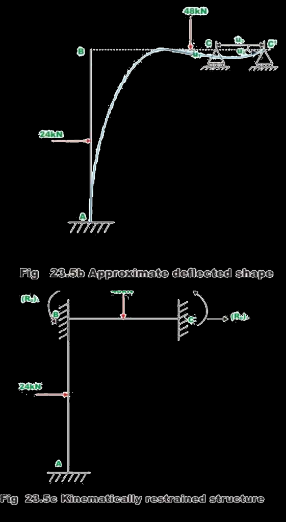
177 Example Analyze the plane frame shown in Fig.23.5a by the direct stiffness method. Assume that the flexural rigidity for all members is the same. Neglect axial displacements. 177

178 Solution In the first step identify the degrees of freedom of the frame.the given frame has three degrees of freedom (see Fig.23.5b): B. Two rotations as indicated by u 1 and u 2 and C. One horizontal displacement of joint B and C as indicated by u 3. In the next step make all the displacements equal to zero by fixing joints B and C as shown in Fig.23.5c. On this kinematically determinate structure apply all the external loads and calculate reactions corresponding to unknown joint displacements.thus, Next calculate stiffness coefficients. Apply unit rotation along u 1 and calculate reactions corresponding to the unknown joint displacements in the kinematically determinate structure (vide Fig.23.5d) 178

179 179

180 180

181 181

182 Similarly, apply a unit rotation along u 2 and calculate reactions corresponding to three degrees of freedom (see Fig.23.5e) k EI k 22 EI k 32 0 (5) Apply a unit displacement along u 3 and calculate joint reactions corresponding to unknown displacements in the kinematically determinate structure. 182

183 Finally applying the principle of superposition of joint forces, yields Now, as there are no loads applied along u 1,u 2 and u 3.Thus the unknown displacements are, Solving u EI 183

184 u 2 EI u EI (8) 184

185 Summary The flexibility coefficient and stiffness coefficients are defined in this section. Construction of stiffness matrix for a simple member is explained. A few simple problems are solved by the direct stiffness method. The difference between the slope-deflection method and the direct stiffness method is clearly brought out. 185

186 TRUSS ANALYSIS An introduction to the stiffness method was given in the previous SECTION. The basic principles involved in the analysis of beams, trusses were discussed. The problems were solved with hand computation by the direct application of the basic principles. The procedure discussed in the previous chapter though enlightening are not suitable for computer programming. It is necessary to keep hand computation to a minimum while implementing this procedure on the computer. In this chapter a formal approach has been discussed which may be readily programmed on a computer. In this lesson the direct stiffness method as applied to planar truss structure is discussed. Plane trusses are made up of short thin members interconnected at hinges to form triangulated patterns. A hinge connection can only transmit forces from one member to another member but not the moment. For analysis purpose, the truss is loaded at the joints. Hence, a truss member is subjected to only axial forces and the forces remain constant along the length of the member. The forces in the member at its two ends must be of the same magnitude but act in the opposite directions for equilibrium as shown in Fig

187 Now consider a truss member having cross sectional area A, Young s modulus of material E, and length of the member L. Let the member be subjected to axial tensile force Fas shown in Fig Under the action of constant axial force F, applied at each end, the member gets elongated by u as shown in Fig

188 The elongation u may be calculated by (vide lesson 2, module 1). FL u AE (24.1) Now the force-displacement relation for the truss member may be written as, AE F u (24.2) L 188

189 F ku (24.3) where is the stiffness of the truss member and is defined as the force required for unit deformation of the structure. The above relation (24.3) is true along the centroidal axis of the truss member. But in reality there are many members in a truss. For example consider a planer truss shown in Fig For each member of the truss we could write one equation of the type Fkualong its axial direction (which is called as local co-ordinate system). Each member has different local co ordinate system. To analyse the planer truss shown in Fig. 24.3, it is required to write force-displacement relation for the complete truss in a co ordinate system common to all members. Such a co-ordinate system is referred to as global co ordinate system. 189

190 LOCAL AND GLOBAL CO-ORDINATE SYSTEM Loads and displacements are vector quantities and hence a proper coordinate system is required to specify their correct sense of direction. Consider a planar truss as shown in Fig In this truss each node is identified by a number and each member is identified by a number enclosed in a circle. The displacements and loads acting on the truss are defined with respect to global co-ordinate system xyz. The same co ordinate system is used to define each of the loads and displacements of all loads. In a global co-ordinate system, each node of a planer truss can have only two displacements: one along x -axis and another along y-axis. The truss shown in figure has eight displacements. Each displacement (degree of freedom) in a truss is shown by a number in the figure at the joint. The direction of the displacements is shown by an arrow at the node. However out of eight displacements, five are unknown. The displacements indicated by numbers 6, 7 and 8 are zero due to support conditions. The displacements denoted by numbers 1-5 are known as unconstrained degrees of freedom of the truss and displacements denoted by 6-8 represent constrained degrees of freedom. In this course, unknown displacements are denoted by lower numbers and the known displacements are denoted by higher code numbers. 190

191 To analyse the truss shown in Fig. 24.4, the structural stiffness matrix K need to be evaluated for the given truss. This may be achieved by suitably adding all the member stiffness matrices k', which is used to express the force-displacement relation of the member in local co-ordinate system. Since all members are oriented at different directions, it is required to transform member displacements and forces from the local co-ordinate system to global co-ordinate system so that a global load-displacement relation may be written for the complete truss. MEMBER STIFFNESS MATRIX Consider a member of the truss as shown in Fig. 24.5a in local co-ordinate system x'y'. As the loads are applied along the centroidal axis, only possible displacements will be along x' -axis. Let the u' 1 andu' 2 be the displacements of truss members in local co-ordinate system i.e.along x'-axis. Here subscript 1 refers to node 1 of the truss member and subscript 2 refers to node 2 of the truss member. Give displacement u' 1 at node 1 of the member in the positive x' direction, keeping all other displacements to zero. This displacement in turn 191

192 induces a compressive force of magnitude EA L u' in the member. Thus, 1 ( ve -ve as it acts in the ve direction for equilibrium). Similarly by giving positive displacements of u' 2 at end 2 of the member, tensile force of magnitude EA u'2 is induced in the member. Thus, L Now the forces developed at the ends of the member when both the displacements are imposed at nodes 1 and 2 respectively may be obtained by method of superposition. Thus (vide Fig. 24.5d) 192

193 Or we can write Thus the member stiffness matrix is This may also be obtained by giving unit displacement at node 1 and holding displacement at node 2 to zero and calculating forces developed at two ends. This will generate the first column of stiffness matrix. Similarly the second column of stiffness matrix is obtained by giving unit displacement at 2 and holding displacement at node 1 to zero and calculating the forces developed at both ends. 193

194 TRANSFORMATION FROM LOCAL TO GLOBAL CO-ORDINATE SYSTEM. Displacement Transformation Matrix A truss member is shown in local and global co ordinate system in Fig Let x' y' z'be in local co ordinate system andxyz be the global co ordinate system. 194

195 The nodes of the truss member be identified by 1 and 2. Let u' 1 and u' 2 be the displacement of nodes 1 and 2 in local co ordinate system. In global co ordinate system, each node has two degrees of freedom. Thus, u 1,v 1 and u 2,v 2 are the nodal displacements at nodes 1 and 2 respectively along x - and y - directions. Let the truss member be inclined to x axis by θ as shown in figure. It is observed from the figure that u' 1 is equal to the projection of u 1 on x' axis plus projection of v 1 on x'-axis. Thus, (vide Fig. 24.7) u' 1 u 1 cosθ v 1 sinθ This may be written as u' 2 u 2 cosθ v 2 sinθ 195

196 Introducing direction cosines lcosθ;msinθ; the above equation is written as In the above equation T is the displacement transformation matrix which transforms the four global displacement components to two displacement component in local coordinate system. 196

197 197

198 Let co-ordinates of node 1 be x 1,y 1 and node 2 be x 2,y 2. Now from Fig. 24.8, (24.11a) (24.11b) (24.11c) Force transformation matrix Let p' 1,p' 2 be the forces in a truss member at node 1 and 2 respectively producing displacements u' 1 and u' 2 in the local co-ordinate system and p 1,p 2,p 3, p 4 be the force in global co-ordinate system at node 1 and 2 respectively producing displacements u 1,v 1 and u 2,v 2 (refer Fig. 24.9a-d). 198

199 199

200 Referring to fig. 24.9c, the relation between p' 1 and p 1, may be written as, p 1 p' 1 cosθ (24.12a) p 2 p' 1 sinθ (24.12b) Similarly referring to Fig. 24.9d, yields p 3 p' 2 cosθ p 4 p' 2 sinθ (24.12c) (24.12d) Now the relation between forces in the global and local co-ordinate system may be written as where matrix p stands for global components of force and matrixp' are the components of forces in the local co-ordinate system. The superscript T stands for the transpose of the matrix. The equation (24.14) transforms the forces in the local co-ordinate system to the forces in global co-ordinate system. This is 200

201 accomplished by force transformation matrix T T. Force transformation matrix is the transpose of displacement transformation matrix. MEMBER GLOBAL STIFFNESS MATRIX From equation (24.6b) we have, p'k 'u' Substituting for p'in equation (24.14), we get p T T k'u' (24.15) 201

202 Making use of the equation (24.10b), the above equation may be written as pt T k't u (24.16) pk u (24.17) Equation (24.17) represents the member load displacement relation in global coordinates and thus k is the member global stiffness matrix. Thus, Each component k ij of the member stiffness matrix kin global co-ordinates represents the force in x-or y-directions at the end irequired to cause a unit displacement along x- or y- directions at end j. 202

203 We obtained the member stiffness matrix in the global co-ordinates by transforming the member stiffness matrix in the local co-ordinates. The member stiffness matrix in global co-ordinates can also be derived from basic principles in a direct method. Now give a unit displacement along x -direction at node 1 of the truss member. Due to this unit displacement (see Fig ) the member length gets changed in the axial direction by an amount equal to l 1 cosθ. This axial change in length is related to the force in the member in two axial directions by 203

204 This force may be resolved along u 1 and v 1 directions. Thus horizontal component of force (24.20b) 204

205 Vertical component of force (24.20c) The forces at the node 2 are readily found from static equilibrium. Thus, (24.20d) (24.20e) The above four stiffness coefficients constitute the first column of a stiffness matrix in the global co-ordinate system. Similarly, remaining columns of the stiffness matrix may be obtained. ANALYSIS OF PLANE TRUSS. Number all the joints and members of a plane truss. Also indicate the degrees of freedom at each node. In a plane truss at each node, we can have two displacements. Denote unknown displacements by lower numbers and known displacements by higher numbers as shown in Fig In the next step evaluate member stiffness matrix of all the members in the global co ordinate 205

206 system. Assemble all the stiffness matrices in a particular order, the stiffness matrix K for the entire truss is found. The assembling procedure is best explained by considering a simple example. For this purpose consider a two member truss as shown in Fig In the figure, joint numbers, member numbers and possible displacements of the joints are shown. 206

207 The area of cross-section of the members, its length and its inclination with the x- axis are also shown. Now the member stiffness matrix in the global co-ordinate system for both the members are given by 207

208 On the member stiffness matrix the corresponding member degrees of freedom and global degrees of freedom are also shown. Note that the member stiffness matrix in global co-ordinate system is derived referring to Fig b. The node 1 and node 2 remain same for all the members. However in the truss, for member 1, the same node (i.e. node 1 and 2 in Fig b) are referred by 2 and 1 respectively. Similarly for member 2, the nodes 1 and 2 are referred by nodes 3 and 4 in the truss. The member stiffness matrix is of the order 4x4. However the truss has six possible displacements and hence truss stiffness matrix is of the order 6x6. Now it is required to put elements of the member stiffness matrix of the entire truss. The stiffness matrix of the entire truss is known as assembled stiffness matrix. It is also known as structure stiffness matrix; as overall stiffness matrix. Thus, it is clear that by algebraically adding the above two stiffness matrix we get global stiffness matrix. For example 208

209 the element k 1 11 of the member stiffness matrix of member 1 must go to location 3,3in the global stiffness matrix. Similarlyk 2 11must go to location3,3 in the global stiffness matrix. The above procedure may be symbolically written as, 209

210 The assembled stiffness matrix is of the order 66. Hence, it is easy to visualize assembly if we expand the member stiffness matrix to 66 size. The missing columns and rows in matrices k 1 and k 2 are filled with zeroes. Thus, 210

211 Adding appropriate elements of first matrix with the appropriate elements of the second matrix, 211

212 If more than one member meet at a joint then the stiffness coefficients of member stiffness matrix corresponding to that joint are added. After evaluating global stiffness matrix of the truss, the load displacement equation for the truss is written as, pk u (24.26) where p is the vector of joint loads acting on the truss, u is the vector of joint displacements and K is the global stiffness matrix. The above equation is known as the equilibrium equation. It is observed that some joint loads are known and some are unknown. Also some displacements are known due to support conditions and some displacements are unknown. Hence the above equation may be partitioned and written as, (24.27) where p k,u k denote vector of known forces and known displacements respectively. And p u,u u denote vector of unknown forces and unknown displacements respectively. Expanding equation 24.27, {p k } k 11 {u u } k 12 {u k } (24.28a) 212

213 { p u } k 21 {u u } k 22 {u k } (24.28b) In the present case (vide Fig a) the known displacements are u 3,u 4,u 5 and u 6. The known displacements are zero due to boundary conditions. Thus, u k 0. And from equation (24.28a), { p k } k 11 {u u } (24.29) Solving {u u }k 11 1 {p k } where k 11 corresponding to stiffness matrix of the truss corresponding to unconstrained degrees of freedom. Now the support reactions are evaluated from equation (24.28b). { p u } k 21 {u u } (24.30) The member forces are evaluated as follows. Substituting equation (24.10b) u 'T u in equation (24.6b)p'k'u', one obtains p'k 'T u (24.31) Expanding this equation, 213

214 Example 24.1 Analyse the two member truss shown in Fig a. Assume EA to be constant for all members. The length of each member is 5m. 214

215 The co-ordinate axes, the number of nodes and members are shown in Fig.24.12b. The degrees of freedom at each node are also shown. By inspection it is clear that the displacement u 3 u 4 u 5 u 6 0. Also the external loads are p 1 5 kn ; p 2 0 kn. (1) Now member stiffness matrix for each member in global co-ordinate system is θ The global stiffness matrix of the truss can be obtained by assembling the two member stiffness matrices. Thus, 215

216 Again stiffness matrix for the unconstrained degrees of freedom is, Writing the load displacement-relation for the truss for the unconstrained degrees of freedom { p k } k 11 {u u } (6) 216

217 The Support reactions are evaluated using equation (24.30). { p u } k 21 {u u } Substituting appropriate values in equation (9), 217

218 by equilibrium of joint (11) 1. Also, p 3 p 5 50 Now force in each member is calculated as follows, Member 1:l0.866 ;m0.5 ;L5m. p'k'u' k't u 218

219 219

220 Summary The member stiffness matrix of a truss member in local co-ordinate system is defined. Suitable transformation matrices are derived to transform displacements and forces from the local to global co-ordinate system. The member stiffness matrix of truss member is obtained in global co-ordinate system by suitable transformation. The system stiffness matrix of a plane truss is obtained by assembling member matrices of individual members in global co-ordinate system. In the end, a few plane truss problems are solved using the direct stiffness matrix approach. \ 220

221 DIRECT STIFFNESS METHOD: BEAMS In the earlier section, a few problems were solved using stiffness method from fundamentals. The procedure adopted therein is not suitable for computer implementation. In fact the load displacement relation for the entire structure was derived from fundamentals. This procedure runs into trouble when the structure is large and complex. However this can be much simplified provided we follow the procedure adopted for trusses. In the case of truss, the stiffness matrix of the entire truss was obtained by assembling the member stiffness matrices of individual members. In a similar way, one could obtain the global stiffness matrix of a continuous beam from assembling member stiffness matrix of individual beam elements. Towards this end, we break the given beam into a number of beam elements. The stiffness matrix of each individual beam element can be written very easily. For example, consider a continuous beam ABCD as shown in Fig. 27.1a. The given continuous beam is divided into three beam elements as shown in Fig. 27.1b. It is noticed that, in this case, nodes are located at the supports. Thus each span is treated as an individual beam. However sometimes it is required to consider a node between support points. This is done whenever the cross sectional area changes suddenly or if it is required to calculate vertical or rotational displacements at an intermediate point. Such a division is shown in Fig. 27.1c. If the axial deformations are neglected then each node of the beam will have two degrees of freedom: a vertical displacement (corresponding to shear) and a rotation (corresponding to bending moment). In Fig. 27.1b, numbers enclosed in a circle represents beam numbers. The beam ABCD is divided into three beam members. Hence, there are four nodes and eight degrees of freedom. The possible displacement degrees of freedom of the beam are also shown in the figure. Let us use lower numbers to denote unknown degrees of freedom (unconstrained degrees of freedom) and higher numbers to denote known (constrained) degrees of freedom. Such a method of identification is adopted in this course for the ease of imposing boundary conditions directly on the structure stiffness matrix. However, one could number sequentially as shown in Fig. 27.1d. This is preferred while solving the problem on a computer. 221

222 222

223 In the above figures, single headed arrows are used to indicate translational and double headed arrows are used to indicate rotational degrees of freedom. BEAM STIFFNESS MATRIX. Fig shows a prismatic beam of a constant cross section that is fully restrained at ends in local orthogonal co-ordinate system x'y'z'. The beam ends are denoted by nodes j and k. The x' axis coincides with the centroidal axis of the member with the positive sense being defined from j to k. Let L be the length of the member, A area of cross section of the member and I zz is the moment of inertia about z' axis. 223

224 Two degrees of freedom (one translation and one rotation) are considered at each end of the member. Hence, there are four possible degrees of freedom for this member and hence the resulting stiffness matrix is of the order 44. In this method counterclockwise moments and counterclockwise rotations are taken as positive. The positive sense of the translation and rotation are also shown in the figure. Displacements are considered as positive in the direction of the coordinate axis. The elements of the stiffness matrix indicate the forces exerted on the member by the restraints at the ends of the member when unit displacements are imposed at each end of the member. Let us calculate the forces developed in the above beam member when unit displacement is imposed along each degree of freedom holding all other displacements to zero. Now impose a unit displacement along y' axis at j end of the member while holding all other displacements to zero as shown in Fig. 27.3a. This displacement causes both shear and moment in the beam. The restraint actions are also shown in the figure. By definition they are elements of the member stiffness matrix. In particular they form the first column of element stiffness matrix. In Fig. 27.3b, the unit rotation in the positive sense is imposed at j end of th beam while holding all other displacements to zero. The restraint actions are shown in the figure. The restraint actions at ends are calculated referring to tables given in lesson 224

225 In Fig. 27.3c, unit displacement along y' axis at end k is imposed and corresponding restraint actions are calculated. Similarly in Fig. 27.3d, unit rotation about z' axis at end k is imposed and corresponding stiffness coefficients are calculated. Hence the member stiffness matrix for the beam member is The stiffness matrix is symmetrical. The stiffness matrix is partitioned to separate the actions associated with two ends of the member. For continuous beam problem, if the supports are unyielding, then only rotational degree of freedom 225

226 shown in Fig is possible. In such a case the first and the third rows and columns will be deleted. The reduced stiffness matrix will be, Instead of imposing unit displacement along y'at j end of the member in Fig. 27.3a, apply a displacement u' 1 along y'at j end of the member as shown in Fig. 27.5a, holding all other displacements to zero. Let the restraining forces developed be denoted by q 11,q 21,q 31 and q

227 The forces are equal to, q k u' ; q k u' ; q 31 k 31 u' 1 ; q 41 k 41 u' 1 (27.3) Now, give displacements u' 1,u' 2,u' 3 and u' 4 simultaneously along displacement degrees of freedom 1,2,3 and 4 respectively. Let the restraining forces developed at member ends be q 1,q 2,q 3 and q 4 respectively as shown in Fig. 27.5b along respective degrees of freedom. Then by the principle of superposition, the force displacement relationship can be written as, This may also be written in compact form as, qku' (27.5) 227

228 BEAM (GLOBAL) STIFFNESS MATRIX. The formation of structure (beam) stiffness matrix from its member stiffness matrices is explained with help of two span continuous beam shown in Fig. 27.6a. Note that no loading is shown on the beam. The orthogonal co-ordinate system xyz denotes the global co-ordinate system. 228

229 For the case of continuous beam, the x - and x' - axes are collinear and other axes ( y and y', z and z' ) are parallel to each other. Hence it is not required to transform member stiffness matrix from local co-ordinate system to global coordinate system as done in the case of trusses. For obtaining the global stiffness matrix, first assume that all joints are restrained. The node and member numbering for the possible degrees of freedom are shown in Fig 27.6b. The continuous beam is divided into two beam members. For this member there are six possible degrees of freedom. Also in the figure, each beam member with its displacement degrees of freedom (in local co ordinate system) is also shown. Since the continuous beam has the same moment of inertia and span, the member stiffness matrix of element 1 and 2 are the same. They are, The local and the global degrees of freedom are also indicated on the top and side of the element stiffness matrix. This will help us to place the elements of the element stiffness matrix at the appropriate locations of the global stiffness matrix. The continuous beam has six degrees of freedom and hence the stiffness matrix is of the order 6 X 6. Let K denotes the continuous beam stiffness matrix of order 6 X 6. From Fig. 27.6b, K may be written as, 229

230 The 4 x 4 upper left hand section receives contribution from member 1 (AB) and 4 x 4 lower right hand section of global stiffness matrix receives contribution frommember 2. The element of the global stiffness matrix corresponding to global degrees of freedom 3 and 4 [overlapping portion of equation 27.7] receives element from both members 1 and 2. Formation of load vector. Consider a continuous beam ABC as shown in Fig

231 We have two types of load: member loads and joint loads. Joint loads could be handled very easily as done in case of trusses. Note that stiffness matrix of each member was developed for end loading only. Thus it is required to replace the member loads by equivalent joint loads. The equivalent joint loads must be evaluated such that the displacements produced by them in the beam should be the same as the displacements produced by the actual loading on the beam. This is evaluated by invoking the method of superposition. 231

232 The loading on the beam shown in Fig. 27.8(a), is equal to the sum of Fig. 27.8(b) and Fig. 27.8(c). In Fig. 27.8(c), the joints are restrained against displacements and fixed end forces are calculated. In Fig. 27.8(c) these fixed end actions are shown in reverse direction on the actual beam without any load. Since the beam in Fig. 27.8(b) is restrained (fixed) against any displacement, the displacements produced by the joint loads in Fig. 27.8(c) must be equal to the displacement produced by the actual beam in Fig. 27.8(a). Thus the loads shown 232

233 in Fig. 27.8(c) are the equivalent joint loads.let, p 1,p 2,p 3,p 4,p 5 and p 6 be the equivalent joint loads acting on the continuous beam along displacement degrees of freedom 1,2,3,4,5 and 6 respectively as shown in Fig. 27.8(b). Thus th global load vector is, 233

234 Solution of equilibrium equations After establishing the global stiffness matrix and load vector of the beam, the load displacement relationship for the beam can be written as, PK u (27.9) where Pis the global load vector, u is displacement vector and K is the global stiffness matrix. This equation is solved exactly in the similar manner as discussed in the lesson 24. In the above equation some joint displacements are known from support conditions. The above equation may be written as displacements. And p u, u u denote respectively vector of unknown forces and unknown displacements respectively. Now expanding equation (27.10), 234

235 { p k } k 11 {u u } k 12 {u k } (27.11a) { p u } k 21 {u u } k 22 {u k } (27.11b) Since u k is known, from equation 27.11(a), the unknown joint displacements can be evaluated. And support reactions are evaluated from equation (27.11b), after evaluating unknown displacement vector. Let R 1,R 3 and R 5 be the reactions along the constrained degrees of freedom as shown in Fig. 27.9a. Since equivalent joint loads are directly applied at the supports, they also need to be considered while calculating the actual reactions. Thus, The reactions may be calculated as follows. The reactions of the beam shown in Fig. 27.9a are equal to the sum of reactions shown in Fig. 27.9b, Fig. 27.9c and Fig. 27.9d. 235

236 236

237 237

238 In the next lesson few problems are solved to illustrate the method so far discussed. Summary In this lesson the beam element stiffness matrix is derived from fundamentals. Assembling member stiffness matrices, the global stiffness matrix is generated. The global load vector is defined. The global load-displacement relation is written for the complete beam structure. The procedure to impose boundary conditions on the load-displacement relation is discussed. With this background, one could analyse continuous beam by the direct stiffness method. 238

239 In the last lesson, the procedure to analyse beams by direct stiffness method has been discussed. No numerical problems are given in that lesson. In this lesson, few continuous beam problems are solved numerically by direct stiffness method. Example 1 Analyse the continuous beam shown in Fig. 28.1a. Assume that the supports are unyielding. Also assume that EI is constant for all members. The numbering of joints and members are shown in Fig. 28.1b. The possible global degrees of freedom are shown in the figure. Numbers are put for the unconstrained degrees of freedom first and then that for constrained displacements. The given continuous beam is divided into three beam elements Two degrees of freedom (one translation and one rotation) are considered at each end of the member. In the above figure, double headed arrows denote rotations and single headed arrow represents translations. In the given problem some displacements are zero, i.e., u 3 u 4 u 5 u 6 u 7 u 8 0 from support conditions. In the case of beams, it is not required to transform member stiffness matrix from local co-ordinate system to global co-ordinate system, as the two co-ordinate system are parallel to each other. 239

240 First construct the member stiffness matrix for each member. This may be done from the fundamentals. However, one could use directly the equation (27.1) given in the previous lesson and reproduced below for the sake convenience. The degrees of freedom of a typical beam member are shown in Fig. 28.1c. Here equation (1) is used to generate element stiffness matrix. Member 1:L4m, node points 1-2. The member stiffness matrix for all the members are the same, as the length and flexural rigidity of all members is the same. 240

241 On the member stiffness matrix, the corresponding global degrees of freedom are indicated to facilitate assembling. Member 2:L4m, node points 2-3. Member 3:L4m, node points

242 The assembled global stiffness matrix of the continuous beam is of the order 8 x 8. The assembled global stiffness matrix may be written as, Now it is required to replace the given members loads by equivalent joint loads. The equivalent loads for the present case is shown in Fig. 28.1d. The displacement degrees of freedom are also shown in Fig. 28.1d. 242

243 hus the global load vector corresponding to unconstrained degree of freedom is, Writing the load displacement relation for the entire continuous beam, 243

244 where pis the joint load vector, u is displacement vector. 244

245 We know that u 3 u 4 u 5 u 6 u 7 u 8 0. Thus solving for unknowns u 1 and u 2, yields Thus displacements are, The unknown joint loads are given by, 245

246 The actual reactions at the supports are calculated as, Member end actions for element 1 Member end actions for element 2 246

247 247

248 Member end actions for element 3 Example 2 Analyse the continuous beam shown in Fig. 28.2a. Assume that the supports are unyielding. Assume EI to be constant for all members. 248

249 The numbering of joints and members are shown in Fig. 28.2b. The global degrees of freedom are also shown in the figure. The given continuous beam is divided into two beam elements. Two degrees of freedom (one translation and one rotation) are considered at each end of the member. In the above figure, double headed arrows denote rotations and single headed arrow represents translations. Also it is observed that displacements u 3 u 4 u 5 u 6 0from support conditions. First construct the member stiffness matrix for each member. Member 1:L4m, node points 1-2. The member stiffness matrix for all the members are the same, as the length and flexural rigidity of all members is the same. On the member stiffness matrix, the corresponding global degrees of freedom are indicated to facilitate assembling. Member 2: L4m, node points 2-3. The assembled global stiffness matrix of the continuous beam is of order 66. The assembled global stiffness matrix may be written as, 249

250 Now it is required to replace the given members loads by equivalent joint loads. The equivalent loads for the present case is shown in Fig. 28.2c. The displacement degrees of freedom are also shown in figure. 250

251 251

252 Thus the global load vector corresponding to unconstrained degree of freedom is, Writing the load displacement relation for the entire continuous beam, 252

253 We know that u 3 u 4 u 5 u 6 0. Thus solving for unknowns u 1 and u 2, yields 253

254 The actual support reactions are, Member end actions for element 1 Member end actions for element 2 PLANE FRAMES In the case of plane frame, all the members lie in the same plane and are interconnected by rigid joints. The internal stress resultants at a crosssection of a plane frame member consist of bending moment, shear force and an axial force. The significant deformations in the plane frame are only flexural and axial. In this lesson, the analysis of plane frame by direct stiffness matrix method is discussed. Initially, the stiffness matrix of the plane frame member is derived in its local coordinate axes and then it is transformed to global co-ordinate system. In the case of plane frames, members are oriented in different directions and hence before forming the global stiffness matrix it is necessary to refer all the member stiffness matrices to the same set of axes. This is achiev ed by transfo rmatio n of forces and displac ement s to global coordinat e syste m. MEMB ER STIFFN ESS MATRI X FOR PLANE FRAME S Consid er a memb er of a plane frame as shown in Fig. 30.1a in the memb er coordinat e syste 254

255 m x'y'z'. The global orthogonal set of axes xyzis also shown in the figure. The frame lies in the xy plane. The member is assumed to have uniform flexural rigidity EI and uniform axial rigidity EA for sake of simplicity. The axial deformatio n of member will be considered in the analysis. The possible displaceme nts at each node of the member are: translation in x' - and y' - direction and rotation about z' - axis. Thus the frame members have six (6) degrees of freedom and are shown in Fig.30.1a. The forces acting on the member at end j and k are shown in Fig. 30.1b. The relation between axial displacement and axial forces is derived in chapter 24. Similarly the relation between shear force, bending moment with translation along y' axis and rotation about z' axis are given in lesson 27. Combining them, we could write the loaddisplacement relation in the local co-ordinate axes for the plane frame as shown in Fig 30.1a, b as, 255

256 This may be succinctly written as where k' is the member stiffness matrix. The member stiffness matrix can also be generated by giving unit displacement along each q possible displacement degree of ' freedom one at a time and calculating resulting restraint actions. k ' TRANSFORMATION FROM LOCAL TO GLOBAL CO-ORDINATE u SYSTEM ' Displacement transformation matrix of the plane frame member a u' 4,u' 5,u' 6 be respectively di coordinate system x'y'z'. Si displac ement s of ends j and k of the memb er in global coordinat e syste m. In plane frame the members are oriented in different directions and hence it is necessary to transform stiffness matrix of individual members from local to global coordinate system before formulating the global stiffness matrix by assembly. In Fig. 30.2a the plane frame member is shown in local coordinate axes x y z and in Fig. 30.2b, the plane frame is shown in global coordinate axes xyz. Two ends 256

257 Fig.30.2a and b, one could relate u' 1,u' 2,u' 3 to u 1,u 2,u 3 as, u' 1 u 1 cosθ u 2 sinθ (3 u' 2 u 1 sinθ u 2 cosθ (3 u' 3 u 3 (3 This may be written as, Let θ be the angle by which the member is inclined to global x -axis. From Where, lcosθ and msinθ. This may be written in compact form as, (30.3b) u't u In the above equation, T is defined as the displacement transformation matrix and it transforms the six global displacement components to six displacement components in local co-ordinate axes. Again, if the coordinate of node j is x 1, y 1 and coordinate of nodek 257

258 are x 2,y 2, then, 258

259 Force displacement matrix Let q' 1, q' 2, q' 3 and q' 4, q' 5, q' 6 be respectively the forces in member at nodes j and k as shown in Fig. 30.3a in local coordinate system. p 1,p 2,p 3 and p 4, p 5, p 6 are the forces in members at node j and k respectively as shown in Fig. 30.3b in the global coordinate system. Now from Fig 30.3a and b, p 1 q' 1 cosθ - q' 2 sinθ (30.5a) 259

260 p 2 q' 1 sinθ q' 2 cosθ (30.5b) 260

261 p 3 q' 3 (30.5c) Thus the forces in global coordinate system can be related to forces in local coordinate system by Where, lcosθ and msinθ. This may be compactly written as, p T T q' (30.6b) Member global stiffness matrix From equation (30.1b), we have q 'k 'u ' 261

262 Substituting the above value of q' in equation (30.6b) results in, pt T k'u' (30.7) Making use of equation (30.3b), the above equation may be written as or pt T k't u (30.8) pk u (30.9) The equation (30.9) represents the member load-displacement relation in global coordinate system. The global member stiffness matrix k is given by, k T T k 'T (30.10) 262

263 After transformation, the assembly of member stiffness matrices is carried out in a similar procedure as discussed for truss. Finally the global load-displacement equation is written as in the case of continuous beam. Few numerical problems are solved by direct stiffness method to illustrate the procedure discussed. Example 30.1 Analyze the rigid frame shown in Fig 30.4a by direct stiffness matrix method. Assume E200GPa;I ZZ m 4 and A0.04m 2. The flexural rigidity EI and axial rigidity EA are the same for both the beams. Solution: The plane frame is divided in to two beam elements as shown in Fig. 30.4b. The numbering of joints and members are also shown in Fig. 30.3b. Each node has three degrees of freedom. Degrees of freedom at all nodes are also shown in the figure. Also the local degrees of freedom of beam element are shown in the figure as inset. 263

264 264

265 Formulate the element stiffness matrix in local co-ordinate system and then transform it to global co-ordinate system. The origin of the global co-ordinate system is taken at node 1. Here the element stiffness matrix in global coordinates is only given. Member 1:L6m;θ90node points 1-2;l0andm1. 265

266 266

267 The load vector corresponding to unconstrained degrees of freedom is (vide 30.4d), In the given frame constraint degrees of freedom are u 1,u 2,u 3,u 7,u 8,u 9. Eliminating rows and columns corresponding to constrained degrees of freedom from global stiffness matrix and writing load-displacement relationship for only unconstrained degree of freedom, 267

268 Example 30.2 Analyse the rigid frame shown in Fig 30.5a by direct stiffness matrix method. Assume E200 GPa ;I ZZ m 4 and A0.01m 2. The flexural rigidity EI and axial rigidity EA are the same for all beams. 268

269 Solution: The plane frame is divided in to three beam elements as shown in Fig. 30.5b. The numbering of joints and members are also shown in Fig. 30.5b. The possible degrees of freedom at nodes are also shown in the figure. The origin of the global co- ordinate system is taken at A (node 1). 269

270 Now formulate the element stiffness matrix in local co-ordinate system and then transform it to global co-ordinate system. In the present case three degrees of freedom are considered at each node. 270

271 271

272 272

273 273

274 The load vector corresponding to unconstrained degrees of freedom is, In the given frame, constraint (known) degrees of freedom are u 1,u 2,u 3,u 10,u 11,u 12. Eliminating rows and columns corresponding to constrained degrees of freedom from global stiffness matrix and writing load displacement relationship, 274

275 Let R 1,R 2,R 3,R 10,R 11,R 12 be the support reactions along degrees of freedom 1, 2, 3,10,11,12 respectively. Support reactions are calculated by 275

276 Unit 5: INFLUENCE LINES FOR INDETERMINATE BEAMS DEFINITION INFLUENCE LINES Influence lines are important in thedesign of structures that resist large live loads.shear and moment diagrams are important in determining the maximum internal force in a structure.if a structure is subjected to a live or moving load, the variation in shear andmoment is best described using influencelines. An influence line represents the variation of the reaction, shear, moment, or deflection at a specific point in a member as a concentrated force moves over the member. Once the influence line is drawn, the location of the live load which will cause the greatest influence on the structure can be found very quickly.therefore, influence lines are important in the design of a structure where the loads move along the span (bridges, cranes, conveyors, etc.). Although the procedure for constructing an influence line is rather simple, it is importantto remember the difference between constructing an influence line and constructing a shear or moment diagram.influence lines represent the effect of amoving load only at a specified point on a member, whereas shear and moment diagrams represent the effect of fixed loads at allpoints along the member. Procedure for determining theinfluence line at a pointpfor anyfunction (reaction, shear, or moment). 1. Place a unit load (a load whose magnitude is equal to one) at a point, x, along the member. 2. Use the equations of equilibrium to find the value of the function (reaction, shear, or moment) at a specific point P due the concentrated load at x. 3. Repeat steps 1 and 2 for various values of x over the whole beam. 4. Plot the values of the reaction, shear, or moment for the member. Construction of Influence Lines using Equilibrium Methods The most basic method of obtaining influence line for a specific response parameter is to solve the static equilibrium equations for various locations of the unit load. The general procedure for constructing an influence line is described below. 1. Define the positive direction of the response parameter under consideration through a free body diagram of the whole system. 276

277 2..For a particular location of the unit load, solve for the equilibrium of the whole system and if required, as in the case of an internal force, also for a part of the member to obtain the response parameter for that location of the unit load.this gives the ordinate of the influence line at that particular location of the load. 3.Repeat this process for as many locations of the unit load as required to determine the shape of the influence line for the whole length of the member. It is often helpful if we can consider a generic location (or several locations) x of the unit load. 4.Joining ordinates for different locations of the unit load throughout the length of the member,we get the influence line for that particular response parameter. The following three examples show how to construct influence lines for a support reaction, a shear force and a bending moment for the simply supported beam AB. Example.1 Draw the influence line for E6.1. (vertical reaction at A ) of beam AB in Fig. Solution: Free body diagram of AB : 277

278 So the influence line of : Example 6.2 Draw the influence line for AB in Fig. E6.2. (shear force at mid point) of beam Solution: 278

279 For So the influence line for v c 279

280 Example 6.3 Draw the influence line for (bending moment at ) for beam AB in Fig. E6.3. Solution: For 280

281 For So, the influence of M D : MÜLLER BRESLAU PRINCIPLE FOR QUALITATIVE INFLUENCE LINES In 1886, Heinrich Müller Breslau proposed a technique to draw influence lines quickly. The Müller Breslau Principle states that the ordinate value of an influence line for any function on any structure is proportional to the ordinates of the deflected shape that is obtained by removing the restraint corresponding to the function from the structure and introducing a force that causes a unit displacement in the positive direction. Let us say, our objective is to obtain the influence line for the support reaction at A for the beam shown in Figure

282 Simply supported beam First of all remove the support corresponding to the reaction and apply a force (Figure 38.2) in the positive direction that will cause a unit displacement in the direction of R A. The resulting deflected shape will be proportional to the true influence line (Figure 38.3) for the support reaction at A. Figure 38.2: Deflected shape of beam 282

283 Figure 38.3: Influence line for support reaction A The deflected shape due to a unit displacement at A is shown in Figure 38.2 and matches with the actual influence line shape as shown in Figure Note that the deflected shape is linear, i.e., the beam rotates as a rigid body without any curvature. This is true only for statically determinate systems. Similarly some other examples are given below. Here we are interested to draw the qualitative influence line for shear at section C of overhang beam as shown in Figure Figure 38.4: Overhang beam 283

284 As discussed earlier, introduce a roller at section C so that it gives freedom to the beam in vertical direction as shown in Figure Now apply a force in the positive direction that will cause a unit displacement in the direction of V C. The resultant deflected shape is shown in Figure Again, note that the deflected shape is linear. Figure 38.6 shows the actual influence, which matches with the qualitative influence. Figure 38.5: Deflected shape of beam 284

285 Figure 38.6: Influence line for shear at section C In this second example, we are interested to draw a qualitative influence line for moment at C for the beam as shown in Figure Figure 38.7: Beam structure In this example, being our objective to construct influence line for moment, we will introduce hinge at C and that will only permit rotation at C. Now apply moment in the positive direction that will cause a unit rotation in the direction of M c. The deflected shape due to a unit rotation at C is shown in Figure 38.8 and matches with the actual shape of the influence line as shown in Figure

286 Figure 38.8: Deflected shape of beam Figure 38.9: Influence line for moment at section C Maximum shear in beam supporting UDLs If UDL is rolling on the beam from one end to other end then there are two possibilities. Either Uniformly distributed load is longer than the span or uniformly distributed load is shorter than the span. Depending upon the length of the load and span, the maximum shear in beam supporting UDL will change. Following section will discuss about these two cases. It should be noted that for maximum values of shear, maximum areas should be loaded. UDL LONGER THAN THE SPAN Let us assume that the simply supported beam as shown in Figure is loaded with UDL of w moving from left to right where the length of the load is longer than the span. The influence lines for reactions R A, R B and shear at section C located at x from support A will be as shown in Figure 38.11, 286

287 38.12 and respectively. UDL of intensity w per unit for the shear at supports A and B will be given by Figure 38.10: Beam Structure Figure 38.11: Influence line for support reaction at A 287