Selected Analytical Methods for Well and Aquifer Evaluation

Transcription

1 BULLETIN 49 STATE OF ILLINOIS DEPARTMENT OF REGISTRATION AND EDUCATION Selected Analytical Methods for Well and Aquifer Evaluation by WILLIAM C. WALTON ILLINOIS STATE WATER SURVEY URBANA 1962

2 STATE OF ILLINOIS HON. OTTO KERNER, Governor DEPARTMENT OF REGISTRATION AND EDUCATION WILLIAM SYLVESTER WHITE, Director BOARD OF NATURAL RESOURCES AND CONSERVATION WILLIAM SYLVESTER WHITE, Chairman ROGER ADAMS, Ph.D., D.Sc., LL.D., Chemistry ROBERT H. ANDERSON, B.S., Engineering THOMAS PARK, Ph.D., Biology WALTER H. NEWHOUSE, Ph.D., Geology CHARLES E. OLMSTED, Ph.D., Botany WILLIAM L. EVERITT, E.E., Ph.D., University of Illinois DELYTE W. MORRIS, Ph.D., President, Southern Illinois University Funds derived from University of Illinois administered grants and contracts were used to produce this report. STATE WATER SURVEY DIVISION WILLIAM C. ACKERMANN, Chief URBANA 1962 Second Printing 1967 Third Printing 1969 Fourth Printing 1977 Fifth Printing 1983 (Sixth Printing )

3 Contents Abstract... 1 Introduction... 1 Part 1. Analysis of geohydrologic parameters... 3 Hydraulic properties... 3 Aquifer tests... 3 Drawdown... 3 Leaky artesian formula... 4 Nonleaky artesian formula... 6 Water-table conditions... 6 Partial penetration... 7 Modified nonleaky artesian formula... 8 Leaky artesian constant-drawdown formula Nonleaky artesian drain formula Specific-capacity data Statistical analysis Flow-net analysis Geohydrologic boundaries Image-well theory Barrier boundary Law of times Aquifer-test data Recharge boundary Aquifer-test data Percentage of water diverted from source of recharge Time required to reach equilibrium Multiple boundary systems Primary and secondary image wells Recharge Flow-net analysis Ground-water and hydrologic budgets Part 2. Analysis of yields of wells and aquifers Model aquifers and mathematical models Records of past pumpage and water levels Computation by electronic digital computer Well characteristics Well loss Collector wells Well design criteria Screened wells Spacing of wells Part 3. Illustrative examples of analyses Barometric efficiency of a well Aquifer-test data under leaky artesian conditions Aquifer-test data under nonleaky artesian conditions Aquifer-test data under water-table conditions Specific-capacity data Statistical analysis Yields of deep sandstone wells and the effects of shooting Effects of acid treatment Flow-net studies Coefficient of transmissibility Coefficient of vertical permeability Aquifer-test data under boundary conditions Barrier boundaries Recharge boundary Recharge rates Area of influence of pumping Flow-net analysis Leakage through confining beds Ground-water and hydrologic budgets i PAGE

4 PAGE Model aquifer and mathematical model for Arcola area Evaluation of several aquifers in Illinois Chicago region Taylorville area Tallula area Assumption area Pekin area Well loss Sand and gravel well Bedrock wells Collector well data Design of sand and gravel well Conclusions Acknowledgments Selected references Appendix A. Values of W ( u, r/b ) Appendix B. Values of K o ( r/b ) Appendix C. Values of W ( u ) Appendix D. Values of G ( λ, r w /B) Appendix E. Values of D ( u )q Appendix F. Selected conversion constants and factors Illustrations FIGURE ii 1 Nonleaky artesian drain type curve Graphs of specific capacity versus coefficient of transmissibility for a pumping period of 2 minutes Graphs of specific capacity versus coefficient of transmissibility for a pumping period of 10 minutes Graphs of specific capacity versus coefficient of transmissibility for a pumping period of 60 minutes Graphs of specific capacity versus coefficient of transmissibility for a pumping period of 8 hours Graphs of specific capacity versus coefficient of transmissibility for a pumping period of 24 hours Graphs of specific capacity versus coefficient of transmissibility for a pumping period of 180 days Graphs of specific capacity versus well radius (A) and pumping period (B) Diagrammatic representation of the image-well theory as applied to a barrier boundary Generalized flow net showing flow lines and potential lines in the vicinity of a discharging well near a barrier boundary Diagrammatic representation of the image well theory as applied to a recharge boundary Generalized flow net showing flow lines and potential lines in the vicinity of a discharging well near a recharge boundary Graph for determination of percentage of pumped water being diverted from a source of recharge Plans of image-well systems for several wedge shaped aquifers Plans of image-well systems for selected parallel boundary situations Plan of image-well system for a rectangular aquifer Illustrative data input format for digital computer analysis of a mathematical model Abbreviated flow diagram for digital computer analysis of a mathematical model Effect of atmospheric pressure fluctuations on the water level in a well at Savoy Map showing location of wells used in test near Dieterich Generalized graphic logs of wells used in test near Dieterich PAGE

5 FIGURE 22 Time-drawdown graph for well 19 near Dieterich Distance-drawdown graph for test near Dieterich Map showing location of wells used in test at Gridley Generalized graphic logs of wells used in test at Gridley Time-drawdown graph for well 3 at Gridley Time-drawdown graph for well 1 at Gridley Map showing location of wells used in test near Mossville Generalized graphic logs of wells used in test near Mossville Time-drawdown graph for well 15 near Mossville Distance-drawdown graph for test near Mossville Areal geology of the bedrock surface in DuPage County Thickness of dolomite of Silurian age in DuPage County Specific capacity frequency graphs for dolomite wells in DuPage County Specific capacity frequency graphs for the units penetrated by dolomite wells in DuPage County Estimated specific capacities of dolomite wells in DuPage County Specific capacity frequency graphs for dolomite wells in northeastern Illinois Specific capacities of wells uncased in the Glenwood-St. Peter Sandstone (A) and the Prairie du Chien Series, Trempealeau Dolomite, and Franconia Formation (B) in northeastern Illinois Specific capacities of wells uncased in the Cambrian-Ordovician Aquifer, theoretical (A) and actual (B) in northeastern Illinois Relation between the specific capacity of a well and the uncased thickness of the Glenwood-St. Peter Sandstone (A) and the uncased thickness of the Mt. Simon Aquifer (B) Thickness of the Glenwood-St. Peter Sandstone in northeastern Illinois Step-drawdown test data showing the results of acid treatment of dolomite wells in DuPage County Cross sections of the structure and stratigraphy of the bedrock and piezometric profiles of the Cambrian-Ordovician Aquifer in northeastern Illinois Piezometric surface of Cambrian-Ordovician Aquifer in northeastern Illinois in Thickness of the Maquoketa Formation in northeastern Illinois Piezometric surface of Cambrian-Ordovician Aquifer in northern Illinois, about 1864 (A); and decline in artesian pressure in Cambrian-Ordovician Aquifer, (B) Map showing location of wells used in test near St. David Generalized graphic logs of wells used in test near St. David Time-drawdown graph for well l-60 near St. David Time-drawdown graph for well 2-60 near St. David Map showing location of wells used in test at Zion Generalized graphic logs of wells used in test at Zion Lake stage and water levels in wells during test at Zion Distance-drawdown graphs for test at Zion Piezometric surface of the Silurian dolomite aquifer in DuPage County Areas influenced by withdrawals from wells in the Silurian dolomite aquifer in selected parts of DuPage County Estimated recharge rates for the Silurian dolomite aquifer in DuPage County Flow-net analysis of the piezometric surface of the Cambrian-Ordovician Aquifer in northeastern Illinois in Mean daily ground-water stage in Panther Creek basin, Mean daily streamflow in Panther Creek basin, Mean daily precipitation in Panther Creek basin, Rating curves of mean ground-water stage versus ground-water runoff for gaging station in Panther Creek basin Graph showing relation of gravity yield and average period of drainage for Panther Creek basin Map and geologic cross section showing thickness and areal extent of aquifer at Arcola PAGE

6 iv FIGURE 65 Model aquifers and mathematical models for Arcola area (A and B) and Chicago region (C and D) Model aquifers and mathematical models for Taylorville (A and B) and Tallula (C and D) areas Model aquifers and mathematical models for Assumption (A and B) and Pekin (C and D) areas Time-drawdown graph for well near Granite City Generalized graphic logs of wells used in test at Iuka Map showing location of wells used in test at Iuka Time-drawdown graph for well 3 at Iuka Time-drawdown graphs for wells 2 and 4 at Iuka Well-loss constant versus specific capacity, pumping levels are above the top of the Silurian dolomite aquifer in DuPage County Well-loss constant versus specific capacity, pumping levels are below top of the Silurian dolomite aquifer in DuPage County Mechanical analyses of samples of an aquifer at Woodstock Mechanical analyses of samples of an aquifer near Mossville PLATE 1 Nonsteady-state leaky artesian type curves 2 Steady-state leaky artesian type curve 3 Nonleaky artesian type curve 4 Nonsteady-state leaky artesian, constant drawdown, variable discharge type curves Tables TABLE IN POCKET 1 Values of partial penetration constant for observation well Values of partial penetration constant for pumped well Effective radii of collector wells Optimum screen entrance velocities Time-drawdown data for well 19 near Dieterich Distance-drawdown data for test near Dieterich Time-drawdown data for well 1 at Gridley Time-drawdown data for well 3 at Gridley Time-drawdown data for well 15 near Mossville Distance-drawdown data for test near Mossville Results of shooting deep sandstone wells in northern Illinois Results of acid treatment of dolomite wells in DuPage County Coefficients of transmissibility computed from aquifer-test data for the Joliet area Time-drawdown data for test at St. David Distance-drawdown data for test at Zion Recharge rates for the Silurian dolomite aquifer in DuPage County Results of flow-net analysis for area west of Joliet Monthly and annual streamflow, ground-water runoff, and surface runoff in inches, 1951, 1952, and 1956, Panther Creek basin Monthly and annual ground-water evapotranspiration in inches, 1951, 1952, and 1956, Panther Creek basin Results of gravity yield analysis for Panther Creek basin Monthly and annual ground-water recharge and changes in storage in inches, 1951, 1952, and 1956, Panther Creek basin Log of well near Granite City Data for step-drawdown test near Granite City Drawdowns and pumping rates for well 1 near Granite City Time-drawdown data for test at Iuka PAGE PAGE

7 Selected Analytical Methods for Well and Aquifer Evaluation by William C. Walton Abstract The practical application of selected analytical methods to well and aquifer evaluation problems in Illinois is described in this report. The subject matter includes formulas and methods used to quantitatively appraise the geohydrologic parameters affecting the water-yielding capacity of wells and aquifers and formulas and methods used to quantitatively appraise the response of wells and aquifers to heavy pumping. Numerous illustrative examples of analyses based on actual field data are presented. The aquifer test is one of the most useful tools available to hydrologists. Analysis of aquifertest data to determine the hydraulic properties of aquifers and confining beds under nonleaky artesian, leaky artesian, water table, partial penetration, and geohydrologic boundary conditions is discussed and limitations of various methods of analysis are reviewed. Hydraulic properties are also estimated with specific-capacity data and maps of the water table or piezometric surface. The role of individual units of multiunit aquifers is appraised by statistical analysis of specificcapacity data. The influence of geohydrologic boundaries on the yields of wells and aquifers is determined by means of the image-well theory. The image-well theory is applied to multiple boundary conditions by taking into consideration successive reflections on the boundaries. Several methods for evaluating recharge rates involving flow-net analysis and hydrologic and ground-water budgets are described in detail. Well loss in production wells is appraised with step-drawdown test data, and well screens and artificial packs are designed based on the mechanical analysis of the aquifer. Optimum well spacings are estimated taking into consideration aquifer characteristics and economics. Emphasis is placed on the quantitative evaluation of the practical sustained yields of wells and aquifers by available analytical methods. The actual ground-water condition is simulated by a model aquifer having straight-line boundaries, an effective width, length, and thickness, and sometimes a confining bed with an effective thickness. The hydraulic properties of the model aquifer and its confining bed, if present, the image-well theory, and appropriate ground-water formulas are used to construct a mathematical model which provides a means of evaluating the performance of wells and aquifers. Records of past pumpage and water levels establish the validity of this mechanism as a model of the response of an aquifer to heavy pumping. Introduction During the last few years it has been more fully realized that refined quantitative answers are needed concerning available ground-water resources and their management. Utilization of aquifers continues to accelerate to meet the needs of irrigation, industrial, urban, and suburban expansion. As ground-water development intensifies, well owners become more interested in the response of aquifers to heavy pumping whereas initially they were concerned largely with the delineation and exploration of aquifers. Competition for available sources has brought about an awareness that one of the principal problems confronting hydrologists is resource management. Before ground-water resources can be managed they must be quantitatively appraised. In ever increasing numbers engineers and geologists are being called upon to estimate how much ground water is available for development and what will be the consequences of exploitation. Ground-water users are continually asking for suggestions as to how available resources can be properly managed. The advice of hydrologists concerning proper well design is often sought. The development of ground-water resources has reached a stage wherein it is highly desirable that the voluminous material in the well and aquifer evaluation field be assembled and briefed in order that engineers and geologists actively engaged in quantitative studies can have available a ready reference. This report is concerned primarily with a brief description of the analytical methods presently used by the Illinois State Water Survey in evaluating wells and aquifers and supersedes Report of Investigation 25. The principles set forth will be applicable, with slight modifica- 1

8 tion, to many parts of the United States and the world. This report is by no means a substitute for the many exhaustive treatises on ground-water hydrology but rather is intended to be a handbook describing formulas and methods commonly used by hydrologists. A comprehensive bibliography is presented containing references to the literature germane to ground-water resource evaluation that may be used to expand the reader s understanding of subject matter. The formulas and analytical methods available to hydrologists are almost unlimited in number, and the discussion of all of them would necessitate several volumes and unwarranted duplications. A selection has therefore been made to include formulas and analytical methods most frequently applied to actual field problems in Illinois. The derivations and proofs of formulas have been eliminated, and formulas are presented in their developed form. The application and limitations of formulas and methods are discussed in detail. A consistent nomenclature has been adopted with clarity and general usage as criteria. This report will find its field of greatest use in aiding the systematic appraisal of ground-water resource problems by professional and practicing engineers, geologists, and well contractors. The subject matter has been arranged in three major parts: 1) formulas and methods used to quantitatively appraise the geologic and hydrologic parameters affecting the water-yielding capacity of wells and aquifers, 2) formulas and methods used to quantitatively appraise the response of wells and aquifers to heavy pumping, and 3) illustrative examples of analyses based on actual field data collected by the Illinois State Water Survey. 2

9 Part 1. Analysis of Geohydrologic Parameters This section describes methods used to evaluate hydraulic properties of aquifers and confining beds, the influence of geohydrologic boundaries on drawdowns in wells, and recharge to aquifers. Analyses of aquifer-test data, specific-capacity data, flownet data, and hydrologic and ground-water budget data are discussed. Hydraulic Properties The coefficients of permeability or transmissibility, storage, and vertical permeability are the major hydraulic properties of aquifers and confining beds upon which the foundation of quantitative ground-water studies is based. The rate of flow of ground water in response to a given hydraulic gradient is dependent upon the permeability of the aquifer. The field coefficient of permeability P is defined as the rate of flow of water, in gallons per day, through a cross-sectional area of 1 square foot of the aquifer under a hydraulic gradient of 1 foot per foot at the prevailing temperature of the water. A related term, the coefficient of transmissibility T, indicates the capacity of an aquifer as a whole to transmit water and is equal to the coefficient of permeability multiplied by the saturated thickness of the aquifer m, in feet. The coefficient of transmissibility is defined as the rate of flow of water, in gallons per day, through a vertical strip of the aquifer 1 foot wide and extending the full saturated thickness under a hydraulic gradient of 1 foot per foot at the prevailing < temperature of the water. The rate of vertical leakage of ground water through a confining bed in response to a given vertical hydraulic gradient is dependent upon the vertical permeability of the confining bed. The field coefficient of vertical permeability P is defined as the rate of vertical flow of water, in gallons per day, through a horizontal cross-sectional area of 1 square foot of the confining bed under a hydraulic gradient of 1 foot per foot at the prevailing temperature of the water. The storage properties of an aquifer are expressed by its coefficient of storage S, which is defined as the volume of water the aquifer releases from or takes into storage per unit surface area of the aquifer per unit change in the component of head normal to that surface. Under artesian conditions, when the piezometric surface is lowered by pumping, water is derived from storage by the compaction of the aquifer and its associated beds and by expansion of the water itself, while the interstices remain saturated. Under water-table conditions, when the water table is lowered by pumping, ground water is derived from storage mainly by the gravity drainage of the interstices in the portion of the aquifer unwatered by the pumping. Under artesian conditions and for granular or loosely cemented aquifers reasonably free from clay beds, the coefficient of storage is a function of the elasticity of water and the aquifer skeleton, as expressed in the following equation (see Jacob, 1950): S = ( p γmß/144) [1 + (ø/pβ )] (1) where: S = coefficient of storage, fraction p = porosity, fraction m = saturated thickness of aquifer, in ft ß = reciprocal of the bulk modulus of elasticity of water, in sq in./lb ø = reciprocal of the bulk modulus of elasticity of aquifer skeleton, in sq in./lb γ = specific weight of water, in lb/cu ft Recognizing that for practical purposes γ = 62.4 lb/cu ft and ß = 3.3x10 6 sq in./lb, the fraction of storage attributable to expansibility of the water S w is given by the following equation: S w = 1.4x10 6 (pm) (2) Aquifer Tests The hydraulic properties of aquifers and confining beds may be determined by means of aquifer tests, wherein the effect of pumping a well at a known constant rate is measured in the pumped well and in observation wells penetrating the aquifer. Graphs of drawdown versus time after pumping started, and/or of drawdown versus distance from the pumped well, are used to solve formulas which express the relation between the hydraulic properties of an aquifer and its confining bed, if present, and the lowering of water levels in the vicinity of a pumped well. Drawdown TO determine drawdown, the water-level trend before pumping started is extrapolated through the pumping period, and differences between extrapolated stages of the water level that would have been observed if the well had not been pumped and water levels measured during the pumping period are computed. Drawdown is not determined from the water level that was measured just prior to the start of the aquifer test. Before water-level data are 3

10 used to determine hydraulic properties they must be adjusted for any pumping-rate changes in nearby production wells. Water levels in wells in artesian aquifers are affected by fluctuations in atmospheric pressure. As the atmospheric pressure increases the water level falls, and as the atmospheric pressure decreases the water level rises. The ratio of the change in water level in a well to the change in atmospheric pressure is known as the barometric efficiency of the well and is usually expressed as a percentage. Barometers are generally calibrated in inches of mercury and changes in atmospheric pressure must be converted from inches of mercury to feet of water before the barometric efficiency of a well can be computed. The conversion is readily expressed as: inches of mercury x 1.13 = feet of water Equations for the barometric efficiency of a well and for the change in water level in response to an atmosphericpressure change are as follows: B.E. = ( W/ B) 100 (3) W = [B.E. ( B)]/100 (4) where: B.E. = barometric efficiency, in per cent W = change in water level resulting from a change in atmospheric pressure, in ft B = change in atmospheric pressure, in ft of water Drawdown data must be adjusted for atmospheric-pressure changes before they are used to determine hydraulic properties. Changes in the time-rate of drawdown due to atmospheric-pressure fluctuations may be mistaken for evidence of geohydrologic boundary conditions. A time interval during which water levels are not affected by pumping changes is selected. Barometer readings, converted to feet of water, are inverted and plotted on plain coordinate paper, together with water-level data for the pumped and observation wells. Prominent barometric fluctuations are used to compare changes in water level caused by changes in atmospheric pressure. The amount of rise in water level as a result of a decrease in atmospheric pressure and the amount of decline in water level as a result of an increase in atmospheric pressure are calculated. The barometric efficiency can then be computed with equation 3. Drawdown data are adjusted for atmospheric-pressure changes occurring during an aquifer test by obtaining a record of atmospheric-pressure fluctuations and using equation 4. Water levels in wells near surface bodies of water are often affected by surface-water stage fluctuations either because of a loading effect or a hydraulic connection between the surface-water body and the aquifer. As the surfacewater stage rises the water level rises, and as the surfacewater stage declines the water level falls. The ratio of the change in the water level in a well to the change in surfacewater stage in the case of a loading effect is known as the tidal efficiency, and the ratio of the change in the water level in a well to the change in surface-water stage in the case where a hydraulic connection exists between the surface-water body and the aquifer is known as the river efficiency. Equations for the tidal and river efficiencies of a well and for the change in water level in response to a surfacewater stage change are as follows: T.E. = ( W/ R ) 100 (5) W = [T.E. ( R)]/100 (6) R.E. = ( W / R) 100 (7) W = [ R.E.( R)]/100 (8) where: T.E. = tidal efficiency, in per cent R.E. = river effciency, in per cent W = change in water level resulting from a change in surface-water stage, in ft R = change in surface-water stage, in ft The tidal or river efficiency can be computed and drawdown data can be adjusted for surface-water stage changes occurring during an aquifer test by obtaining a record of surface-water stage fluctuations during the test and using equations 5 and 6 or 7 and 8. The application or the removal of heavy loads in the vicinity of some artesian wells causes changes in their water levels. Fluctuations in water levels (Roberts and Romine, 1947) sometimes occur when railroad trains or trucks pass aquifer test sites. Drawdown data must be adjusted for these changes in loading before they are used to determine the hydraulic properties of aquifers and confining beds. Leaky Artesian Formula The data collected during aquifer tests may be analyzed by means of the leaky artesian formula (Hantush and Jacob, 1955a). The leaky artesian formula may be written as: s = (114.6Q/T) W ( u,r/b) (9) where: u= and r/b = 2693r²S/Tt (10) (11) s = drawdown in observation well, in ft r = distance from pumped well to observation well, in ft Q = discharge, in gallons per minute (gpm) t = time after pumping started, in minutes (min) T = coefficient of transmissibility, in gallons per day per foot (gpd/ft) S = P = coefficient of storage of aquifer, fraction coefficient of vertical permeability of confining bed, in gallons per day per square foot (gpd/sq ft) m = thickness of confining bed through which leakage occurs, in ft W ( u,r/b) is read as the well function for leaky artesian 4

11 aquifers (Hantush, 1956) and is defined by the following equation: or, evaluating the integral, where: K o(r/b) = modified Bessel function of the second kind and zero order and I o (r/b) = modified Bessel function of the first kind and zero order. The leaky artesian formula was developed on the basis of the following assumptions: that the aquifer is infinite in areal extent and is of the same thickness throughout; that it is homogeneous and isotropic; that it is confined between an impermeable bed and a bed through which leakage can occur; that the coefficient of storage is constant; that water is released from storage instantaneously with a decline in head; that the well has an infinitesimal diameter and penetrates the entire thickness of the formation; that leakage through the confining bed into the aquifer is vertical and proportional to the drawdown; that the hydraulic head in the deposits supplying leakage remains more or less uniform; that the flow is vertical in the confining bed and horizontal in the aquifer; and that the storage in the confining bed is neglected. In cases where leakage is derived in part by the reduction in storage in the confining bed, aquifer-test data can be analyzed with formulas derived by Hantush (1960). The leaky artesian formula may be solved by the following method (Walton, 1960a) which is a modification of the type curve graphical method devised by Theis and described by Jacob (1940). Values of W ( u,r/b) in terms of the practical range of u and r/b were given by Hantush (1956) and are presented in tabular form in appendix A of this report. Values of W (u,r/b) are plotted against values of l/u on logarithmic paper and a family of leaky artesian type curves is constructed as shown in plate 1. Values of s plotted on logarithmic paper of the same scale as the type curves against values of t describe a time-drawdown field data curve that is analogous to one of the family of leaky artesian type curves. The time-drawdown field data curve is superposed on the family of leaky artesian type curves, keeping the W(u,r/B) axis parallel with the s axis and the l/u axis parallel with the t axis. In the matched position a point at the intersection of the major axes of the leaky artesian type curve is selected and marked on the time-drawdown field data curve (the point also may be selected anywhere on the type curve). The coordinates of this common point (match point) W (u,r/b), l/u, s, and t are substituted into equations 9, 10, and 11 to determine the hydraulic properties of the aquifer and confining bed. T is calculated using equation 9 with the W (u,r/b) and s coordinates. S is determined using equation 10, the calculated value of T, and the l/u and t coordinates of the match point. The coefficient of storage must exceed S w in equation 2 or the analysis is incorrect. The value of r/b used to construct the particular leaky artesian type curve found to be analogous to the timedrawdown field data curve is substituted in equation 11 to determine P. Interpretations of aquifer-test data based solely on time drawdown graphs are weak. Distance-drawdown data complement time-drawdown data, and the hydraulic properties of the aquifer and confining bed can be determined from distance-drawdown field data curves (radial profiles of cones of depression). Values of W ( u,r/b) are plotted against values of r/b on logarithmic paper and a family of leaky artesian type curves is constructed. Values of s plotted against values of r on logarithmic paper of the same scale as the type curves describe a distance-drawdown field data curve that is analogous to one of the family of leaky artesian type curves. The distance-drawdown field data curve is superposed on the family of leaky artesian type curves, keeping the W(u,r/B) axis parallel with the s axis and the r/b axis parallel with the r axis. The distance-drawdown field data curve is matched to one of the family of leaky artesian type curves. In the matched position a point at the intersection of the major axes of the leaky artesian type curve is selected and marked on the distance-drawdown field data curve. Match-point coordinates W (u,r/b), r/b, s, and r are substituted in equations 9 and 11 to determine the coefficients of transmissibility and vertical permeability. The value of u/r² used to construct the particular leaky artesian type curve found to be analogous to the distancedrawdown field data curve is substituted in equation 10 to compute S. Under steady-state leaky artesian conditions, that is when time-drawdown data fall on the flat portions of the family of leaky artesian type curves indicating that discharge is balanced by leakage, the cone of depression is described by the following formula (see Jacob, 1946a): s = [229QK 0 ( r/b)]/t (12) where: (13) s = drawdown in observation well, in ft r = distance from pumped well to observation well, in ft Q = discharge, in gpm T = coefficient of transmissibility, in gpd/ft P = coefficient of vertical permeability of confining bed, in gpd/sq ft m = thickness of confining bed through which leakage occurs, in ft K o (r/b) = modified Bessel function of the second kind and zero order Jacob (1946a) devised the following graphical method 5

12 for determining values of the parameters T and P under steady-state leaky artesian conditions. A steady-state leaky artesian type curve is prepared by plotting values of K o (r/b) against values of r/b on logarithmic paper as shown in plate 2. Values of K o (r/b) in terms of the practical range of r/b are given in appendix B. Aquifer-test data collected under steady-state conditions are plotted on logarithmic paper of the same scale as the type curve with r as the abscissa and s as the ordinate to describe a distancedrawdown field data curve. A match of the two curves is obtained by superposing the distance-drawdown field data curve over the steady-state leaky artesian type curve, keeping the axes of the two graphs parallel. In the matched position a point at the intersection of the major axes of the steady-state leaky artesian type curve is selected and marked on the distance-drawdown field data curve. Match-point coordinates K o (r/b), r/b, s, and r are substituted into equations 12 and 13 to determine T and P. The coefficient of storage cannot be computed by use of the steady-state leaky artesian type curve because, under such conditions of flow, the entire yield of the well is derived from leakage sources only. Nonleaky Artesian Formula If leakage through the confining bed into the aquifer is not measurable or the confining bed is missing, equation 9 becomes s = (114.6Q/T) W (u) (14) where: and u = s= Q = T = r = 2693r²S/Tt drawdown in observation well, in ft discharge, in gpm coefficient of transmissibility, in gpd/ft distance from observation well to pumped well, in ft (15) S = coefficient of storage, fraction t = time after pumping started, in min Equation 14 is the nonequilibrium formula introduced by Theis (1935) and will be referred to hereafter as the nonleaky artesian formula. W(u) is the well function for nonleaky artesian aquifers (see Wenzel, 1942). If leakage is not measurable during the aquifer test or the confining bed is missing, the time-drawdown field data curve will be analogous to the nonleaky artesian type curve which is shown in plate 1 as the outside curve of the family of leaky artesian type curves. The time-drawdown field data curve and the nonleaky artesian type curve are matched 6 and match point coordinates W(u), l/u, s, and t are substituted into equations 14 and 15 to determine T and S. The coefficients of transmissibility and storage can also be computed with distance-drawdown data under nonleaky artesian conditions. Values of W(u), given by Wenzel (1942) and presented in tabular form in appendix C, were plotted against values of u on logarithmic paper to obtain the nonleaky artesian type curve in plate 3. Values of s measured at the same time in several wells at various distances from the pumped well are plotted against the squares of the respective distances on logarithmic paper of the same scale as the type curve to obtain a distance-drawdown field data curve. The distance-drawdown field data curve is superposed on the nonleaky artesian type curve keeping the axes of the two graphs parallel. In the matched position a point at the intersection of the major axes of the nonleaky artesian type curve is selected and marked on the distance-drawdown field data curve. Match-point coordinates W(u), u, s, and r ² are substituted into equations 14 and 15 to determine T and S. Water-Table Conditions The methods described in preceding paragraphs pertain to leaky artesian and nonleaky artesian conditions. The nonleaky artesian formula can be applied to the results of aquifer tests made with wells in water-table aquifers under certain limiting conditions. The nonleaky artesian formula was developed in part on the basis of the following assumptions: that the coefficient of storage is constant and that water is released from storage instantaneously with a decline in head. Under water-table conditions, water is derived largely from storage by the gravity drainage of the interstices in the portion of the aquifer unwatered by the pumping. The gravity drainage of water through stratified sediments is not immediate and the nonsteady flow of water towards a well in an unconfined aquifer is characterized by slow drainage of interstices. Thus, the coefficient of storage varies and increases at a diminishing rate with the time of pumping. The important effects of gravity drainage are not considered in the nonleaky artesian formula and that formula does not describe completely the drawdown in wells especially during short periods of pumping. With long periods of pumping the effects of gravity drainage become small and time-drawdown and distance-drawdown curves conform closely to the nonleaky artesian type curve. According to Boulton (1954a) whether or not the nonleaky artesian formula gives a good approximation of the drawdown in a well under water-table conditions depends on the distance of the observation well from the pumped well r, the hydraulic properties of the aquifer, the saturated thickness of the aquifer m, and a dimensionless time factor. He further implies that the nonleaky artesian formula describes the drawdown in wells with sufficient accuracy for practical purposes when the time factor is greater than 5 and r is between about 0.2 m and 6 m. By substituting a numerical value equal to 5 for Boulton s time factor, the following equation can be derived: t wt = 37.4S y m/p (16) where: t wt = approximate time after pumping starts when the

13 S y = P = m = application of the nonleaky artesian formula to the results of aquifer tests under water-table conditions is justified, in days specific yield, fraction coefficient of permeability, in gpd/sq ft saturated thickness of aquifer, in ft The above equation is not valid when r is less than about 0.2 m or greater than about 6 m. For observation wells at great distances from the pumped well, t wt must be something greater than that given by equation 16 before the nonleaky artesian formula can be applied to aquifer-test data. It is evident that t wt is small if an aquifer is thin and very permeable. For example, t wt is about 1 hour if an observation well is close to a pumped well and penetrates an aquifer 30 feet thick with a coefficient of permeability of 5000 gpd/sq ft. In contrast, substituting the data for a thick aquifer of low permeability (m = 200 feet and P = 1000 gpd/sq ft) in equation 16 results in a t wt of about 1.5 days. Gravity drainage of interstices decreases the saturated thickness and therefore the coefficient of transmissibility of the aquifer. Under water-table conditions, observed values of drawdown must be compensated for the decrease in saturated thickness before the data can be used to determine the hydraulic properties of the aquifer. The following equation derived by Jacob (1944) is used to adjust drawdown data for decrease in the coefficient of transmissibility: s' = s (s² /2 m) (17) where: s = drawdown that would occur in an equivalent nonleaky artesian aquifer, in ft s = observed drawdown under water-table conditions, in ft m = initial saturated thickness of aquifer, in ft Under water-table conditions values of drawdown adjusted for decreases in saturated thickness are plotted against the logarithms of values of t to describe a timedrawdown field data curve. The time-drawdown field data curve is superposed on the nonleaky artesian type curve, keeping the axes of the two curves parallel. The time-drawdown field data curve is matched to the nonleaky artesian type curve. Emphasis is placed on late time-drawdown data (usually after several minutes or hours of pumping) because early time-drawdown data are affected by gravity drainage. Match-point coordinates W(u), l/u, s, and t are substituted into equations 14 and 15 to determine T and S. After tentative values of T and S have been calculated, t wt is computed from equation 16. The time t wt is compared with the early portion of data ignored in matching curves. If the type curve is matched to drawdown data for values of time equal to and greater than t wt then the solution is judged to be valid. If the type curve is matched to drawdown data for values of time earlier than t wt then the solution is not correct and the time-drawdown field data curve is re- matched to the nonleaky artesian type curve and the procedures mentioned earlier are repeated until a valid solution is obtained. Gravity drainage is far from complete during the average period (8 to 24 hours) of aquifer tests; therefore, the coefficient of storage computed with data collected under water-table conditions will generally be less than the specific yield of the aquifer and it cannot be used to predict longterm effects of pumping. It should be recognized that the coefficient of storage computed from test results applies largely to the part of the aquifer unwatered by pumping and it may not be representative of the aquifer at lower depths. Partial Penetration Production and observation wells often do not completely penetrate aquifers. The partial penetration of a pumping well influences the distribution of head in its vicinity, affecting the drawdowns in nearby observation wells. The approximate distance r pp from the pumped well beyond which the effects of partial penetration are negligible is given by the following equation (see Butler, 1957): (18) where: m = saturated thickness of aquifer, in ft P h = horizontal permeability of aquifer, in gpd/sq ft P v = vertical permeability of aquifer, in gpd/sq ft According to Hantush (1961), the effects of partial penetration closely resemble the effects of leakage through a confining bed, the effects of a recharge boundary, the effects of a sloping water-table aquifer, and the effects of an aquifer of nonuniform thickness. He outlines methods for analysis of time-drawdown data affected by partial penetration under nonsteady state, nonleaky artesian conditions. In many cases distance-drawdown data can be adjusted for partial penetration according to methods described by Butler (1957). If the pumped well only partially penetrates an aquifer, the cone of depression is distorted and observed drawdowns in observation wells differ from theoretical drawdowns for a fully penetrating well according to the vertical position of the observation well. If the pumped and observation wells are both open in either the top or the bottom portion of the aquifer, the observed drawdown in the observation well is greater than for fully penetrating conditions. If the pumped well is open to the top of the aquifer and the observation well is open to the bottom of the aquifer, or vice versa, the observed drawdown in the observation well is smaller than for fully penetrating conditions. In the case where both the pumped and observation wells are open in the same zone of the aquifer, the following equation (see Butler, 1957) can be used to adjust observed drawdowns in observation wells for the effects of partial penetration: s = C po s pp (19) 7

14 where: s= Cpo = s pp = drawdown in observation well for fully penetrating conditions, in ft partial penetration constant for observation well, fraction observed drawdown for partial penetrating conditions, in ft Table 1. Values of partial penetration constant for observation well α Values of C po for r e /m = Values of Cpo for r e /m = Values of C po for r e /m = Values of C po for r e /m = From Butler (1957 ); adapted from Jacob (1945) Values of Cpo can be obtained from table 1. In table 1, r=distance from pumped well to observation well, in feet; m = saturated thickness of aquifer, in feet; α = fractional penetration; P h =horizontal permeability of aquifer, in gpd/sq ft; P v = vertical permeability of aquifer, in gpd/sq ft; and r e = virtual radius of cone of depression, assumed to be 10,000 feet for artesian conditions and 1000 feet for water-table conditions. In the case where the pumped well penetrates the top of the aquifer and the observation well penetrates the bottom of the aquifer, or vice versa, the following equation (see Butler, 1957) can be used to adjust observed drawdowns for the effects of partial penetration: s = [C po /(2C po 1)]s pp (20) The following equation (see Butler, 1957) can be used to adjust the observed drawdown in a pumped well for the effects of partial penetration: where: s = C pp = s pp = s = C ppspp (21) drawdown for pumped well for fully penetrating conditions, in ft partial penetration constant for pumped well, fraction observed drawdown for partial penetration conditions, in ft Table 2. Values of partial penetration constant for pumped well α , Values of C pp From Butler (1957); based on equation derived by Kozeny (1933) Values of C pp are given in table 2 where r w = nominal radius of well, in feet. Equations 19 through 21 assume steady-state conditions which are not always attained during actual periods of aquifer tests. Tests one day or more in duration are generally long enough to establish steady-state flow in the vicinity of the pumped well and observation wells within the area affected by partial penetration. Equations 19 through 21 give fair results even though steady-state conditions are not attained especially when the aquifer penetrated is of small and known thickness. At best, adjustments for partial penetration by any method can be considered only approximate because the ratio P v /P h is never precisely known. To determine the hydraulic properties of an aquifer with aquifer-test data affected by partial penetration, drawdowns computed with equation 19 or 20 are plotted against the squares of the respective distances to obtain a distancedrawdown field data curve. The distance-drawdown field data curve is superposed on the appropriate type curve (either plate 2 or 3). The two curves are matched and match-point coordinates are substituted into appropriate equations for computation of the hydraulic properties of the aquifer and confining bed, if present. Modified Nonleaky Artesian Formula Jacob (1946b) recognized that when u becomes small (less than, say, 0.01) the sum of the terms in W (u) be- 8

15 yond ln u becomes insignificant. When the pumping period becomes large or when the distance r is small, values of u will be small. When u < = 0.01 then W (u) = ( ln u) and s = (114.6Q/T) ( In u) (22) Equation 22 is the modified nonleaky artesian formula and can be solved graphically (Cooper and Jacob, 1946). Drawdowns in an observation or pumped well are adjusted, if needed, for effects of atmospheric-pressure changes, surface-water stage changes, dewatering, and partial penetration. Values of adjusted drawdown are plotted against the logarithms of time after pumping started on semilogarithmic paper. The time-drawdown field data graph will yield a straight-line graph in the region where u < = The straight-line portion of the time-drawdown field data graph is extrapolated to its intersection with the zero-drawdown axis. The slope of the straight line is used to determine the coefficient of the transmissibility, and the zero-drawdown intercept is used to calculate the coefficient of storage. Expressions for the computations are: T = 264Q/ s (23) S = Tt o /4790r² (24) where: T = coefficient of transmissibility, in gpd/ft S = coefficient of storage, fraction Q = discharge, in gpm s = drawdown difference per log cycle, in ft r = distance from pumped well to observation well, in ft t o = intersection of straight-line slope with zerodrawdown axis, in min The coefficient of storage cannot be determined with any degree of accuracy from data for the pumped well because the effective radius of the pumped well is seldom known and drawdowns in the pumped well are often affected by well losses which cannot be determined precisely. Drawdowns observed at the end of a particular pumping period in two or more observation wells at different distances from the pumped well can be plotted against the logarithms of the respective distances on semilogarithmic paper. The distance-drawdown field data graph will yield a straight-line graph in the region where u < = The straight-line portion of the distance-drawdown graph is extrapolated to its intersection with the zero-drawdown axis. The slope of the straight line is used to determine the coefficient of transmissibility, and the zero-drawdown intercept is used to calculate the coefficient of storage. Expressions for the computations are: T = 528Q/ s (25) S= Tt/4790r o ² (26) where: T = coefficient of transmissibility, in gpd/ft S = coefficient of storage, fraction Q = discharge, in gpm s = drawdown difference per log cycle, in ft r o = intersection of straight-line slope with zerodrawdown axis, in ft t = time after pumping started, in min The straight-line method based on the modified nonleaky artesian formula is popular largely because of its simplicity of application and interpretation; however, as pointed out by Cooper and Jacob (1946), the method is not applicable in some cases and it supplements, rather than supersedes, the type curve method. They state further, the method is designed especially for artesian conditions, but it may be applied successfully to tests of non-artesian aquifers under favorable circumstances. The straight-line method is based on the fact that when u becomes small a plot of drawdown against the logarithm of time after pumping started or distance from the pumped well describes a straight line. A semilogarithmic graph of values of W (u ) and u does not describe a straight line until u < = Deviation from a straight line becomes appreciable when u exceeds about Therefore, a plot of drawdown against the logarithm of time after pumping. started or the logarithm of distance from the pumped well cannot describe a straight line until u becomes small (say less than 0.02). Scattered drawdown data are often interpreted as describing a straight line when actually they plot as a gentle curve. After tentative values of T and S have been calculated, the region of the data where u < = 0.02 should be calculated and compared with the region of data through which the straight line was drawn. The time that must elapse before the straight-line method can be applied to aquifer test data is readily determined from the following equation: t 8l = 1.35x10 5 r 2 S/T (27) where: t 8l = r = time after pumping starts before a semilog timedrawdown or distance-drawdown plot will yield a straight-line graph, in min distance from pumped well to observation well, in ft coefficient of transmissibility, in gpd/ft coefficient of storage, fraction T = S = Inserting the data for an artesian aquifer (S = , T = 17,000 gpd/ft, and r = 100 feet) in equation 27 results in a t 8l of about 8 minutes. In contrast, t 8l is about 2 days for a water-table aquifer (S = 0.2, T = 100,000 gpd/ ft, and r = 100 feet). Although the values of t 8l given above apply only to the particular assumptions made, they do point out that the straight-line method should be used with caution particularly in the water-table aquifer situation. The determination of the storage coefficient by the straight-line method may involve appreciable error. The zero-drawdown intercept is poorly defined where the slope of the semilog plot is small. Intercepts often occur at points where the values of time are very small and minor deviations in extrapolating the straight line will result in large variations in computed values of the coefficient of storage. 9

16 Leaky Artesian Constant-Drawdown Formula In the usual aquifer test the discharge rate of the pumped well is held γ constant and the drawdown varies with time. Hantush (1959b) derived an equation for determining the hydraulic properties of an aquifer and confining bed from an aquifer test in which the discharge varies with time and the drawdown remains constant. The formula describing leaky artesian constant-drawdown variable discharge conditions may be written as: s w = 229Q/[G(l,r w /B)T ] (28) λ = 9.29x10 5 Tt/ r w ²S (29) where: G ( l,r w / B) = (r w / B) [K 1 (r w / B)/K o ( r w / B)] + (4/p ²) exp[ l(r w /B)²] u exp ( lu ²) J o ² ( u) + Y o ²( u ) du u² + (r w /B)² (30) u = T = coefficient of transmissibility, in gpd/ft S = coefficient of storage, fraction Q = discharge, in gpm r w = nominal radius of pumped well, in ft s w = drawdown in pumped well, in ft t = time after discharge started, in min P' = coefficient of vertical permeability of confining bed, in gpd/sq ft m' = thickness of confining bed through which leakage occurs, in ft K 1 (rw / B) = first-order modified Bessel function of the second kind K o (r w / B) = zero-order modified Bessel function of the second kind J o (u ) = zero-order Bessel function of the first kind Y o (u) = zero-order Bessel function of the second kind The equation is based on the same assumptions as those for the leaky artesian equation except that the drawdown is constant and the discharge is variable. G( λ, r w /B) is the well function for leaky artesian aquifers and constant drawdown. Hantush (1959b) gave values of G ( λ, r w / B) in the practical range of λ and r / B. Values of G ( λ, r w / B) given in appendix D were plotted against values of λ on logarithmic paper and a family of leaky artesian constant-drawdown type curves was constructed as shown in plate 4. Values of discharge plotted against values of time on logarithmic paper of the same scale as the type curves describe a timedischarge field data curve that is analogous to one of the family of type curves. The time-discharge field data curve is superposed on the family of type curves, keeping the G ( λ, r w / B) axis parallel with the Q axis and the λ axis parallel with the t axis. The time-discharge field data curve is matched to one of the type curves and a point at the intersection of the major axes of the type curve is selected and marked on the timedischarge field data curve. The coordinates of the match point G ( λ, r w /B), λ, Q, and t are substituted in equations 28 and 29 to determine T and S. T is calculated using equation 28 with the G ( λ, r w / B) and Q match-point coordinates. S is determined using equation 29, the calculated value to T, and the λ and t coordinates of the match point. The value of r /B used to construct the particular type curve found to be analogous to the time-discharge field data curve is substituted in equation 30 to compute P. Nonleaky Artesian Drain Formula In 1938 Theis (in Wenzel and Sand, 1942) developed a formula for determining the hydraulic properties of a nonleaky artesian aquifer with data on the decline in artesian head at any distance from a drain discharging water at a uniform rate. The formula is based on most of the assumptions used to derive the nonleaky artesian formula. In addition, it is assumed that the drain completely penetrates the aquifer and discharges water at a constant rate. The drain formula may be written (Knowles, 1955) as: s = (720Q b X / T ) D (u) q (31) where: and u ² = 2693X²S/Tt (32) s = drawdown at any point in the vicinity of the drain, in ft Q b = constant discharge (base flow) of the drain, in gpm per lineal foot of drain X = distance from drain to point of observation, in ft t = time after drain started discharging, in min T = coefficient of transmissibility, in gpd/ft S = coefficient of storage, fraction Knowles (1955) gave values of D ( u) q for the practical range of values for u (see appendix E). The nonleaky artesian drain type curve in figure 1 was constructed by plotting values of 1/u² against values of D( u ) q on logarithmic graph paper. D ( u ) q is read as the drain function for nonleaky artesian aquifers. Values of drawdown are plotted versus values of time on logarithmic paper having the same log scale as that used to construct the nonleaky artesian drain type curve. The timedrawdown field data curve is superposed over the nonleaky artesian drain type curve, the two curves are matched, and a match point is selected. The coordinates of the match 10

17 11

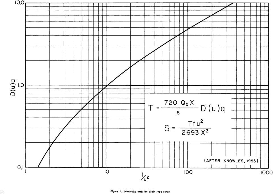
18 point D(u) q, l/u², s, and t are substituted into equations 31 and 32 for computation of T and S. Specific-Capacity Data In many cases, especially in reconnaissance ground-water investigations, the hydraulic properties of an aquifer must be estimated based on well-log, water-level, and specificcapacity data. High specific capacities generally indicate a high coefficient of transmissibility, and low specific capacities generally indicate low coefficients of transmissibility. The specific capacity of a well cannot be an exact criterion of the coefficient of transmissibility because specific capacity is often affected by partial penetration, well loss, and geohydrologic boundaries. In most cases these factors adversely affect specific capacity and the actual coefficient of transmissibility is greater than the coefficient of transmissibility computed from specific-capacity data. Because of the usefulness of rough estimates of T, an examination of the relation between the coefficient of transmissibility and specific capacity is useful. The theoretical specific capacity of a well discharging at a constant rate in a homogeneous, isotropic, nonleaky artesian aquifer infinite in areal extent is from the modified nonleaky artesian formula given by the following equation: Q / s = T /[264 log (Tt /2693r w²s) 65.5] (33) where: Q /s = specific capacity, in gpm/ft Q = discharge in gpm s = drawdown, in ft T = coefficient of transmissibility, in gpd/ft S = coefficient of storage, fraction rw = nominal radius of well, in ft t = time after pumping started, in min The equation assumes that: 1) the well penetrates and is uncased through the total saturated thickness of the aquifer, 2) well loss is negligible, and 3) the effective radius of the well has not been affected by the drilling and development of the well and is equal to the nominal radius of the well. The coefficient of storage of an aquifer can usually be estimated with well-log and water-level data. Because specific capacity varies with the logarithm of l/s, large errors in estimated coefficients of storage result in comparatively small errors in coefficients of transmissibility estimated with specific-capacity data. The relationships between the specific capacity and the coefficient of transmissibility for artesian and water-table conditions are shown in figures 2 through 7. Pumping periods of 2 minutes, 10 minutes, 60 minutes, 8 hours, 24 hours, and 180 days; a radius of 6 inches; and storage coefficients of and 0.02 were assumed in constructing the graphs. These graphs may be used to obtain rough estimates of the coefficients of transmissibility from specificcapacity data. The coefficient of storage is estimated from well-log and water-level data, and a line based on the estimated S is drawn parallel to the lines on one of figures Figure 2. Graphs of specific capacity versus coefficient of transmissibility for a pumping period of 2 minutes Figure 3. Graphs of specific capacity versus coefficient of transmissibility for a pumping period of 10 minutes Figure 4. Graphs of specific capacity versus coefficient of transmissibility for a pumping period of 60 minutes 12

19 2 through 7, depending upon the pumping period. The coefficient of transmissibility is selected from the point of intersection of the S line and the known specific capacity. As shown by equation 33, the specific capacity varies with the logarithm of l/r u ². Large increases in the radius of a well result in comparatively small changes in Q/s. The relationship between specific capacity and the radius of a well assuming T = 17,000 gpd/ft, S = , and t = 1 day is shown in figure 8A. A 30-inch-diameter well has a specific capacity about 8 per cent more than that of a 16-inchdiameter well; a 16-inch-diameter well has a specific capacity about 3 per cent more than that of a 12-inch-diameter well. Figure 5. Graphs of specific capacity versus coefficient of transmissibility for a pumping period of 8 hours Figure 8. Graphs of specific capacity versus well radius (A) and pumping period (B) Figure 6. Graphs of specific capacity versus coefficient of transmissibility for a pumping period of 24 hours Specific capacity decreases with the period of pumping as shown in figure 8B, because the drawdown continually increases with time as the cone of influence of the well expands. For this reason, it is important to state the duration of the pumping period for which a particular value of specific capacity is computed. The graph of specific capacity versus pumping period in figure 8B was constructed by assuming T = 17,000 gpd/ft, S = , and r w = 6 inches. Statistical Analysis The methods of statistical analysis can be of great help in appraising the role of individual units of multiunit aquifers as contributors of water. The productivity of some bedrock aquifers, especially dolomite aquifers, is inconsistent and it is impossible to predict with a high degree of accuracy the specific capacity of a well before drilling at any location. However, the probable range of specific capacities of wells can often he estimated based on frequency graphs. Figure 7. Graphs of specific capacity versus coefficient of Suppose that specific-capacity data are available for wells transmissibility for a pumping period of 180 days penetrating one or several units of a multiunit aquifer and 13

20 it is required to estimate the range in productivity and relative consistency in productivity of the three units. Specific capacities are divided by the total depths of penetration to obtain specific capacities per foot of penetration. Wells are segregated into categories depending upon the units penetrated by wells. Specific capacities per foot of penetration for wells in each category are tabulated in order of magnitude, and frequencies are computed with the following equation derived by Kimball (1946): F = [ m o / (n w +l)]l00 (34) where: m o = the order number n w = total number of wells F = percentage of wells whose specific capacities are equal to, or greater than, the specific capacity of order number m o Values of specific capacity per foot of penetration are then plotted against the percentage of wells on logarithmic probability paper. Straight lines are fitted to the data. If specific capacities per foot of penetration decrease as the depth of wells and number of units penetrated increase, the upper units are more productive than the lower units. Unit-frequency graphs can be constructed from the category-frequency graphs by the process of subtraction, taking into consideration uneven distribution of wells in the categories. The slope of a unit-frequency graph varies with the inconsistency of production, a steeper line indicating a greater range in productivity. Flow-Net Analysis Contour maps of the water table or piezometric surface together with flow lines are useful for determining the hydraulic properties of aquifers and confining beds and estimating the velocity of flow of ground water. Flow lines, paths followed by particles of water as they move through an aquifer in the direction of decreasing head, are drawn at right angles to piezometric surface or water-table contours. If the quantity of water percolating through a given cross section (flow channel) of an aquifer delimited by two flow lines and two piezometric surface or water-table contours is known, the coefficient of transmissibility can be estimated from the following modified form of the Darcy equation: T = Q /IL (35) where: Q = discharge, in gpd T = coefficient of transmissibility, in gpd/ft I = hydraulic gradient, in feet per mile (ft/mi) L = average width of flow channel, in miles (mi) L is obtained from the piezometric surface or water-table map with a map measurer. The hydraulic gradient can be calculated by using the following formula (sec Foley, Walton, and Drescher, 1953): I = c / W a (36) where: I = hydraulic gradient, in ft/mi 14 c = contour interval of piezometric surface or watertable map, in ft and W a = A /L (37) in which A is the area, in square miles, between two limiting flow lines and piezometric surface or water-table contours; and L is the average length, in miles, of the piezometric surface or water-table contours between the two limiting flow lines. If the quantity of leakage through a confining bed into an aquifer, the thickness of the confining bed, area of confining bed through which leakage occurs, and the difference between the head in the aquifer and in the source bed above the confining bed are known, the coefficient of vertical permeability can be computed from the following modified form of the Darcy equation: P' = Q c m / ha c (38) where: P = coefficient of vertical permeability of confining bed, in gpd/sq ft Q c = leakage through confining bed, in gpd m = thickness of confining bed through which leakage occurs, in ft A c = area of confining bed through which leakage occurs, in sq ft h = difference between the head in the aquifer and in the source bed above the confining bed, in ft The velocity of the flow of ground water can be calculated from the equation of continuity, as follows: V = Q /7.48S y A (39) where: V = velocity, in feet per day (fpd) Q = discharge, in gpd A = cross-sectional area of the aquifer, in sq ft S y = specific yield of aquifer, fraction The specific yield converts the total cross-sectional area of the aquifer to the effective area of the pore openings through which flow actually occurs. The discharge Q can be calculated from Darcy s equation as the product of the coefficient of permeability, hydraulic gradient, and cross-sectional area of aquifer or: Q = PIA (40) Substitution of equation 40 in equation 39 results in the expression (see Butler, 1957): V = PI /7.48S y (41) where: V = velocity of flow of ground water, in fpd P = coefficient of permeability, in gpd/sq ft I = hydraulic gradient, in ft/ft S y = specific yield, fraction The range in ground-water velocities is great. Under heavy pumping conditions, except in the immediate vicinity of a pumped well, velocities are generally less than 100 feet