SEASONAL ADJUSTMENT. 1 Introduction. 2 Methodology. 3 X-11-ARIMA and X-12-ARIMA Methods

Transcription

1 SEASONAL ADJUSTMENT 1 Inroducion 2 Mehodology 2.1 Time Series and Is Componens Seasonaliy Trend-Cycle Irregulariy Trading Day and Fesival Effecs 3 X-11-ARIMA and X-12-ARIMA Mehods 3.1 Moving Averages Definiion Symmeric Moving Averages used in X Properies of Moving Averages Symmeric Henderson Moving Averages 3.2 Basic Algorihm of X ARIMA Models 4 Seasonal Adjusmen Procedure a he Cenral Bureau of Saisics 4.1 Prior Adjusmen Facors for Trading Day and Fesival Effecs Explanaory Variables Regression Models for Monhly and Quarerly Series Prior Adjused Original Series 4.2 Seasonal Facors Final Seasonally Adjused Series 4.3 Trend Esimaes Improved Mehod for Trend Esimaion 4.4 Special Issues Concurren Seasonal Adjusmen Seasonal Adjusmen of Composie (Aggregae) Series 5 The Publicaion 5.1 Descripion of he Tables 5.2 Descripion of he Diagrams 5.3 Comparison o he Previous Publicaion 5.4 Bibliography

2 1. Inroducion Socio-economic ime series daa are used for sudying and following he developmens of rends and for deecing he occurrence of urning poins and changes in he direcion of he socio-economic aciviy. This deecion ask is made difficul when he original daa conain no only he fundamenal rend-cycle behavior of ineres, bu also he movemens aribuable o seasonal, rading day, movable holiday and irregular influences. In order o esimae he rend in ime series, seasonal, movable holiday and rading day variaions mus firs be removed and hen irregular influences dampened. This publicaion describes he laes mehods used for seasonal adjusmen a he Cenral Bureau of Saisics (CBS). We also provide here comprehensive informaion regarding more han 400 ime series ha are regularly published by he Bureau. The publicaion is based on he research on ime series analysis carried ou by he Saisical Analysis Secor. In his research, mehods developed in oher leading saisical agencies, academic insiuions and cenral banks around he world are analyzed, new mehods are developed, and hose appropriae o Israeli ime series are applied. In paricular, he prior adjusmen facors are calculaed using he special mehod developed by he CBS for he esimaion of he moving Jewish fesival daes and rading day effecs in Israel. The seasonal facors, and he seasonally adjused series, are calculaed using he X-12-ARIMA (U.S. Census Bureau, 2001) seasonal adjusmen mehod. The esimaion of he rend is carried ou according o an improved mehod based on symmeric Henderson moving averages and an addiional process ha is described in Secion The firs par of he publicaion focuses on a deailed presenaion of our mehodology. In Secion 2 we define a ime series and is componens. In Secion 3 we describe he X-11-ARIMA and X-12-ARIMA seasonal adjusmen mehods. X-12-ARIMA is he laes in he family of he seasonal adjusmen mehods developed over several decades by he U.S. Census Bureau and Saisics Canada. In 2002, we sared he process of implemening his mehod as he sandard program. Since he beginning of 2005, all series are seasonally adjused using his mehod. Secion 4 covers he procedure of seasonal adjusmen a he CBS, ha is, he esimaion of: prior adjusmen facors for rading day and fesival effecs (4.1), seasonal facors (4.2), seasonally adjused series (4.2.1), and rend (Secion 4.3). Finally, we discuss concurren seasonal adjusmen (Secion 4.4.1) and seasonal adjusmen of composie (aggregae) series (Secion 4.4.2). The second par of he publicaion presens ables of he fesival and rading day prior adjusmen facors, and he seasonal facors for he year These are provided for more han 400 ime series ha are currenly published in he Monhly Bullein of Saisics and in oher publicaions of he CBS. The hird par shows diagrams illusraing he original, fesival and rading day adjused, seasonally adjused, and rend series, for he main socio-economic indicaors in Israel s economy for In addiion, diagrams for fesival and rading day, seasonal, and irregular facors, as well as he percenage change on he previous monh (quarer) in he rend are included for he same series and he same period. The appendix presens daa on Jewish fesival daes and working day variaion in Israel for he years

3 2. Mehodology 2.1 Time Series and Is Componens A ime series is a sequence of observaions ordered in ime, X 1, X 2,..., beween imes and +1 being fixed and consan hroughou. X,..., X T ; he inerval The ime series colleced by he CBS are saisical records of a paricular social or economic aciviy, like indusrial producion, person-nighs in ouris hoels, road accidens. They are measured a regular inervals of ime, usually monhly or quarerly, over relaively long periods. This allows he disclosure of paerns of behavior over ime, o analyze hem and place he curren esimaes ino a more meaningful and hisorical perspecive. Noionally, a ime series can be decomposed ino a number of fundamenal componens, each of which has is own disinguishing characer. In a simple model, he original daa a any ime poin (denoed byo ) may be expressed as a funcion f of hree main componens: he seasonaliy ( S ), he rend-cycle ( C ), and he irregulariy ( I ), ha is O = f ( S, C, I ) Diagram 1 shows a graphic represenaion of he original series (non-seasonally adjused series) of Deparures of Israelis Abroad by Air, monhly, from January 2000 o March I can be seen from he diagram ha he series exhibis regular seasonal effec, wih deparures high in summer and low in winer. Depending mainly on he naure of he seasonal movemens of a given series, several differen models can be used o describe he way in which he componens C, S and I are combined o compose he original serieso. There are hree basic seasonal models in which X-12- ARIMA can decompose he series and idenify and remove he seasonaliy. The choice of model depends on wheher i is more appropriae o consider he rend, seasonal and irregular componens o be proporional o each oher or largely independen of each oher. Specifically, he muliplicaive model reas all hree componens as dependen on each oher; ha is, he seasonal oscillaion size increases and decreases wih he level of he series. In conras, he addiive model assumes ha he absolue sizes of he componens of he series are independen of each oher and, in paricular he size of he seasonal oscillaions is independen of he level of he series. The pseudo-addiive model reas he seasonal and irregular componens as independen of each oher bu dependen upon he level of he rend. In he muliplicaive and he pseudo-addiive models, he rend-cycle ( C ) is measured in he same unis as he original series ( O ), and he seasonal ( S ) and irregular componens ( I ) are expressed as percenages, so hey are cenered abou 100. In he addiive model all hree componens are measured in he same unis as he original series and he seasonal and irregular componens vary abou 0. In Diagram 2, hree examples of monhly ime series are presened. For each series, only one seasonal decomposiion model is appropriae

4 Diagram 2.a: Muliplicaive model. This is he mos frequenly used model for ime series. As can be seen in he diagram, he magniude of he seasonal flucuaions is proporional o he level of he series. This model assumes ha he rend, seasonal and irregular componens are represened by a muliplicaive funcion so ha he observed series a ime may be modeled by: O = C S I (1) Alhough mos series a he CBS are adjused muliplicaively here are some excepions. Series ha include exremely small values or zeros canno be adjused using a muliplicaive model, so an addiive or a pseudo-addiive model is used. Diagram 2.b: Addiive model. This is he mos appropriae model for series where he magniude of he seasonal componen does no appear o be affeced by he level of he series. The series is decomposed in his case as follows: O = C + S + I Diagram 2.c: Pseudo-addiive model. This model provides he bes seasonal adjusmen for series wih exreme seasonal variaions ha is some monhs (quarers) having exremely small values or zeros and he remaining monhs (quarers) appearing o have a muliplicaive seasonaliy. The seasonal and irregular componens are expressed in percenages. The model combines he elemens of boh he addiive and muliplicaive models as follows: O = C + C ( S 1) + C ( I 1) = C ( S + I 1) Each one of he hree main componens of he ime series, ha is he seasonaliy ( S ), he rend-cycle ( C ), and he irregulariy ( I ), displays disincly differen characerisics and will be discussed below

5 2.1.1 Seasonaliy ( S ) The seasonal componen represens inra-year, monhly or quarerly, flucuaions ha recur every year wih more or less he same iming and inensiy. Thus, hey creae an annual paern of changes, a seasonal paern. Some examples of his kind of influences are he considerable increase of residens deparing abroad in June, July and Augus, he significan drop in prices of clohing in February-March and Sepember. Causes for seasonal flucuaions include naural facors (climaic variaions: summer, winer, rainfalls), adminisraive or legal measures (saring and ending daes of school year, fiscal year) and social/culural/radiional, and calendar-relaed effecs ha are sable in annual iming (e.g., public fixed holidays such as Chrismas, Valenine s Day). Calendar-relaed - 4 -

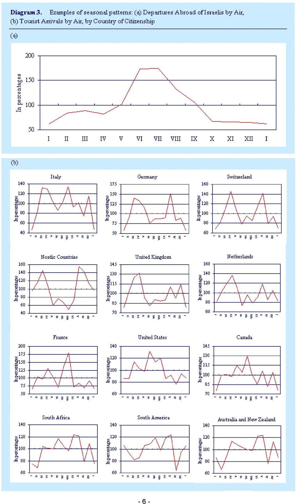
6 sysemaic effecs associaed wih he daes of moving holidays like Passover and he Jewish New Year (Rosh Hashanah) are no seasonal in his sense, because hey occur in differen calendar monhs depending on he daes of he holidays. Diagram 3 presens examples of seasonal paerns: Diagram 3.a illusraes he seasonal paern of one series: Deparures Abroad of Israelis by Air, for The values of he esimaed seasonal componen are called seasonal facors. The seasonal facors, esimaed using he muliplicaive model, are measured on a percenage scale. Facors greaer han 100 percen indicae a high season (he original series is greaer han he rend), and facors less han 100 percen indicae a low season. As he diagram shows, he series exhibis a disincive paern ypically high in June, July and Augus, he monhs mos people ake vacaions, and lower in November, December, January and February. Diagram 3.b shows he differen seasonal paerns of 12 series: monhly series of incoming ourism o Israel by counry of ciizenship, esimaed using he muliplicaive model. I is seen ha he welve seasonal paerns vary subsanially boh in shape and magniude Range of Seasonaliy Seasonal variaion can be very large or relaively small. The difference beween he highes (peak) and he lowes (rough) of he annual seasonal facors, expressed in percenages, is called he range of seasonaliy, and is a measure of he magniude of he seasonal variaion. Using he range of seasonaliy, he Israeli series were classified ino hree groups: a) high seasonaliy (range greaer han 50 %), b) inermediae (20-50 %), and c) low (less han 20%). Diagram 4 illusraes examples for each group. Noe he changes in he values in he y-axis, of he seasonal facors, for each example Sable and Moving Seasonaliy The seasonal paern may be consan or evolve in ime during he analyzed period. If i is consan or remains almos he same in ime, in magniude and shape, hen i is said ha he series presens sable seasonaliy. In he case ha i evolves, ha is he seasonal paern changes gradually over ime, in ampliude, shape, or boh ampliude and shape, i is said ha he series has moving seasonaliy. There are many causes for he laer: seasonal paern may gradually evolve as economic behavior, economic srucures, echnological advances, and insiuional and social arrangemens change. For example, a gradual decrease is observed in he magniude of he seasonal componen for agriculure series caused by echnological changes ha reduce he effec of weaher on growh and sales of fruis and vegeables. In a composie (aggregae) series, ha is he series is composed of sub-series, i may occur due o change in weighs of sub-series

7 - 6 -

8 Table 1 presens he seasonal facors of he monhly series Generaion of Elecriciy (in millions of kilowas per hour), for January 1996 o December The series is decomposed using he muliplicaive model, so he seasonal facors are expressed in percenages. A seasonal facor of denoes ha here is no seasonal effec. The yearly average of he facors is 100.0, meaning ha all he seasonal influences occur during a single year. The able shows ha he series has moving seasonaliy, wih gradual change for almos all monhs in he period The seasonal facors for January decrease monoonically from o and for Augus hey increase from o

9 The seasonaliy becomes more significan in March, June, July, Sepember, Ocober and November, whereas in December he seasonaliy weakens over ime. For he res of he monhs, February, April and May, he seasonal effecs remain nearly he same Trend-Cycle ( C ) Many ime series exhibi a endency o grow or o decrease fairly seadily over quie long periods of ime. This paern is idenified as rend. Anoher inerpreaion of he rend is ha i represens he underlying direcion of he series lasing for many years, and obained afer excluding he seasonal and he irregular influences. The rend capures he long-erm behavior of he series and herefore is movemens are smooh and gradual. A quasi-periodic oscillaion may be someimes observed around he rend, characerized by alernaing periods ha are generally longer han one year, cycles. An example of i is he business cycle, during which he socio-economic aciviy alernaely expands and conracs. The idenificaion of rend has always posed a serious saisical problem. No convenien analyical mehod has been found o separae he long-erm rend from he cycles. Therefore, hey are reaed as a single componen, rend-cycle ( C ). The rend-cycle sems from facors such as populaion growh, echnological developmen, and economic or securiy siuaions. A rend break, or level shif, is defined as an abrup bu susained change in he level of a series. The annual seasonal paern is no changed, bu is simply a a differen level. The reasons for a rend break can be changes in conceps and definiions of a survey, collecion mehod, echnology, economic behavior, legislaion, social radiions, ec. For example, in Israel, due o he securiy siuaion, a srong rend break was deeced as of Ocober 2000 for all series of incoming ourism and person-nighs of ouriss in ouris hoels. Diagram 5 presens an example of he rend-break deeced in he series Touris Arrivals by Air. Trend breaks are a problem for seasonal adjusmen as hey can cause disorions in he esimaes of all componens of he series. Hence, if a rend break is deeced in he daa i should be handled before he seasonal adjusmen. The X-11-ARIMA soluion is o creae a back series ha mainains he seasonal paern in he original daa bu shifs he level so i is consisen wih he new level of he series

10 This new series is used o seasonally adjus he series for he period afer he rend break. For he daa before he rend break he seasonal adjusmen is carried ou as usual. In he X-12- ARIMA mehod, a level shif variable can be included in he model o accoun for a sharp and susained change in he level of he series. In any case, he final seasonally adjused series will show a disconinuiy a he beginning of he rend break. (An explanaion on he seasonal adjusmen mehods is provided in Secion 3) Irregulariy ( I ) This componen represens he variaion remaining afer adjusing he original series for rend and seasonaliy. I comprises hree pars: a) Calendar changes, such as hose associaed wih he moving daes of religious fesivals (which migh simply resul in he ransfer of socio-economic aciviy beween successive monhs like March-April and Sepember-Ocober), changes in he daily (weekday) composiion of monhs of he same year, and beween he same monh of differen years (e.g. he number of Sundays, Mondays). These influences can be esimaed and forecas based on pas experience, since he calendar srucure is known. b) Exreme one-ime evens, such as wars, srikes, special weaher condiions and economic insabiliy. Usually, hese evens canno be forecas and i is difficul o esimae heir effec. c) Residual irregulariy, arising from measuremen errors, response errors and oher errors Trading Day and Fesival Effecs ( P ) As indicaed in Secion 2.1.3, he irregular facors ( I ) may be decomposed ino subcomponens: he changes in he number of rading days and fesival daes (also called calendar effecs), and he remaining irregulariy. Therefore model (1) may be exended as follows: I = P E and hus O = C S P E (2) - 9 -

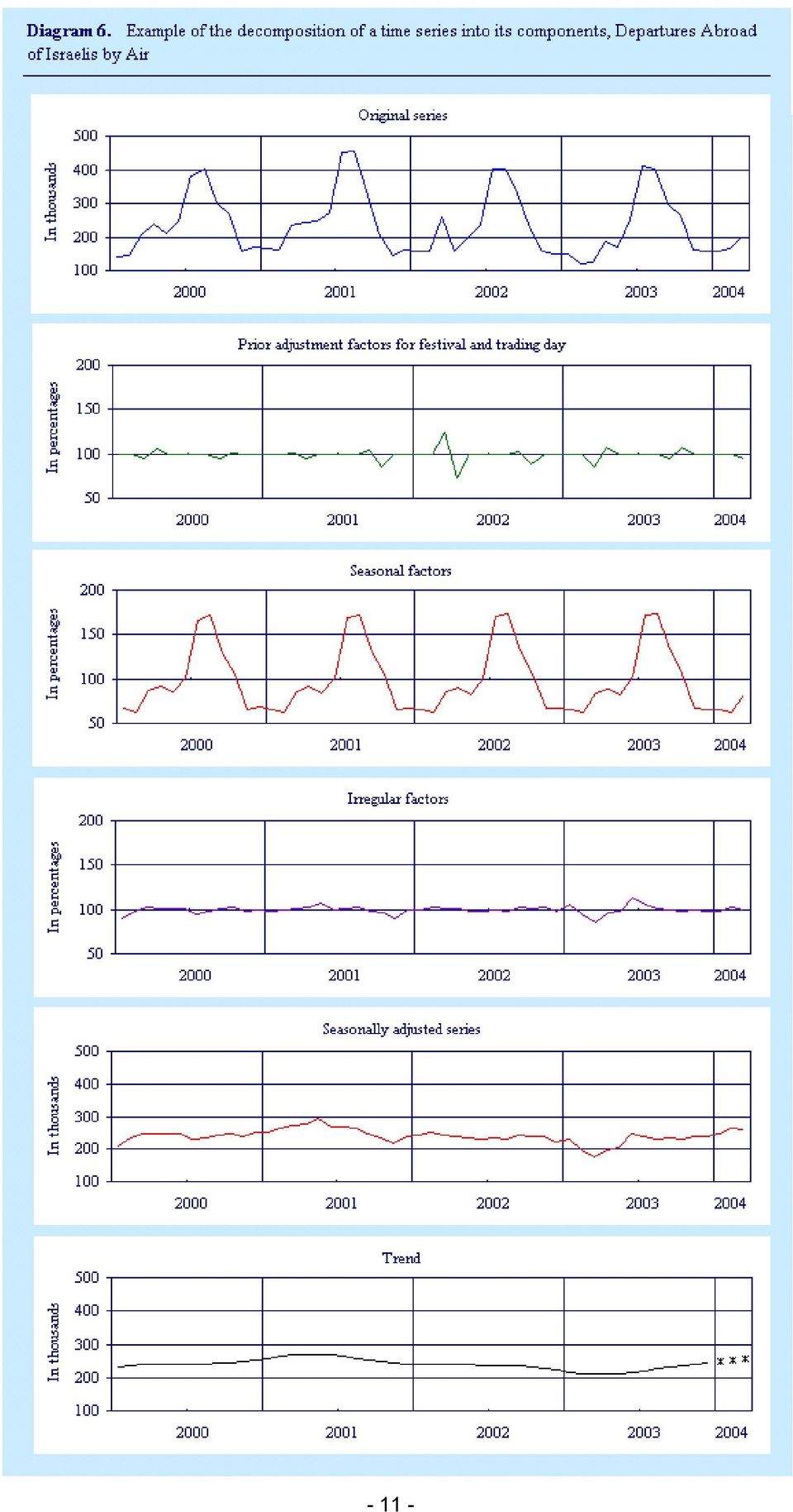
11 where P is he adjusmen facor for he calendar effecs (changes in he fesival daes and he number of rading days in a monh) and E is he residual variaion caused by all oher influences. (For furher explanaion on he esimaion of P, see Secion 4.1). Diagram 6 summarizes he decomposiion of a ime series ino is componens. The series analyzed is Deparures of Israelis Abroad, by Air, and he period presened is January 2000 o March A muliplicaive seasonal model is used for he decomposiion. The diagram provides an illusraion of he meaning of seasonal adjusmen showing separaely he componens of he series, ha is, he prior adjusmen for fesivals and rading day, he seasonal, he irregular and he rend-cycle. The unadjused daa (original series) presens he acual economic evens ha have occurred, while he seasonally adjused daa and he rend-cycle esimae represen an analyical elaboraion of he daa designed o show he underlying movemens ha may be hidden by he fesival and rading day, seasonal and he irregular variaions. These hree ses of daa provide useful informaion abou he economy and hey should be presened o he users. The original series ( O ), of Diagram 1, is shown in he op panel of diagram 6. The prior adjusmen facors for fesival and rading day ( P ), in he second panel, highligh he adjusmens for he Spring and Auumn Jewish holidays, wih a relaively high effec in In ha year boh fesivals daes fell close o heir earlies possible saring dae, ha is, he series is esimaed o be high by 25 % in March and 3% in Sepember, and low in April by 30% and by 10% in Ocober. The seasonal facors ( S ) in he nex panel show, ha he srucure observed in Diagram 3.a for 2003 repeas iself in oher years. Analyzing he seasonaliy of he series i can be seen ha i has high and sable seasonaliy. Tha is, he original daa is higher by 70% in he peak monhs of July and Augus and low by 35% in he winer monhs of November, December, January and February. The irregular facors ( E ), shown in he fourh panel, indicae low unexplained effecs, no larger han 7%. Observe he paricularly srong one-ime exreme irregular effec of 10 % in November 2001, afer he error aack in New York and 15 % in March 2003, he monh ha sared he war in Iraq. In he las wo panels he seasonally adjused series, ( SA ) and he rend ( C ) are displayed. The fifh panel presens he seasonally adjused series. Noice ha i is smooher han he original series as he regular influences of fesival and rading day, and seasonaliy have been removed, alhough he irregular componen sill remains, especially visible in November 2001 and March In order o eliminae also he irregular componen, he rend-cycle is esimaed, using he seasonally adjused daa, hus obaining a smooher an easy inerpreable series ha is presened in he sixh panel

12 - 11 -

13 3. X-11-ARIMA and X-12-ARIMA Mehods The U.S. Census Bureau devised a general approach o seasonal adjusmen in 1965, called he X-11 mehod, which became he sandard mehod used by many governmen saisics offices around he world. A major developmen of he mehod was made by Saisics Canada in 1980, wih he seasonal adjusmen mehod named X-11-ARIMA. Is mos imporan improvemen is ha i allows he user o augmen he observed series, before seasonal adjusmen, wih forecass (and backcass) values from ARIMA models. The use of forecas exensions generally resuls in smaller revisions of he seasonal adjusmens, especially a he end of he series, on average; beer rend esimaion a he end of he series. In addiion, i includes he esimaion of indirec seasonal adjusmen of series ha are aggregae of muliple componen series, and beer diagnosics for assessing he qualiy of he seasonal adjusmen. In 1996, he U.S. Census Bureau developed an enhanced version of he X-11-ARIMA called X-12-ARIMA. X-12-ARIMA s major enhancemens include new X-11-ARIMA adjusmen opions, new and beer diagnosics, new modeling capabiliies especially for handling calendar effecs, and improved user inerface. The basic algorihm of X-11 is common o boh he X-11-ARIMA and X-12-ARIMA mehods. I uses moving averages o esimae he main componens of he series: rend and seasonaliy. Moving averages are essenially weighed averages of he observaions. They are nonparameric, simple and especially flexible in heir applicaion. I is possible o consruc a moving average ha has good properies in erms of rend preservaion, eliminaion of seasonaliy and noise reducion. Secion explains in deail he ypes of moving averages used by he menioned mehods. Finally, i is worh menioning ha he X-11-ARIMA and he new X-12-ARIMA mehods are he mos widely used programs for seasonal adjusmen in governmen saisics offices, some oher organizaions and universiies. In Europe, some governmen agencies and saisics organizaions use he package TRAMO/SEATS, a model-based approach ha is described in Gomez and Maravall (2000). 3.1 Moving Averages There are various ypes of arihmeic averages. In a simple average all he values conribue equally o he average, ha is, hey have an equal weigh in he calculaion. In relaion o ime series daa, an average may be applied o he whole series o produce a single averaged value, or an average may be applied o successive overlapping sub-periods of he series, hereby producing a series of averaged values. In he laer case, he resuls are produced from a simple moving average. For example, applying a 13 simple moving average o a ime series is carried ou as follows: firs calculae he simple average of he firs 13 consecuive observaions, hen move along he series one observaion, dropping ou of he calculaion span he firs observaion and bringing in he foureenh observaion, and calculae he simple average of hese 13 observaions. The process of moving along he series one observaion a a ime and aking he 13-erm average is repeaed, unil here are no furher ime series observaions o bring ino he 13-erm span. A moving average can be of any lengh and can ake on any weighing paern as long as he weighs are posiive and sum o 1. As differen weighing paerns end o give rise o moving averages wih differen characerisics, moving averages are ofen classified on he basis of heir associaed weighing paerns. We menioned above he simple moving average, based on uniform weighs. If he weighs are no uniform he moving average is said o be nonsimple. A moving average may be also described as being eiher symmeric or asymmeric, depending on he form of is weighing paern. In paricular, a moving average is said o be symmeric if he weighing paern used o calculae i is symmeric abou he cener of he averaging span, oherwise i is said o be asymmeric. In a cenered simple moving

14 average, he resuls of applying symmeric moving averages are placed in he cener of each average span, in order no o inroduce phase shifing in he new series Definiion We define a moving average M ( O ) of order (lengh) p + f + 1 and weighs W k as: + f M ( O ) = WO k + k. k= p Thus, he value a ime of he original series is herefore replaced by a weighed average of p pas values of he series, he curren value, and f he fuure values of he series. The quaniy p + f + 1 is called he moving average order. When p = f, ha is when he number of observaions in he pas is he same as he number of observaions in he fuure, he moving average is said o be cenered. If, in addiion, W k = Wk for any k, he moving average M is said o be symmeric; oherwise is said o be asymmeric. Generally, wih a moving average of order p + f + 1 calculaed for ime wih p observaions in he pas and f observaions in he fuure, i will be impossible o smooh ou he firs p observaions and he las f observaions of he series. A composie simple moving average of order P Q is obained by composing wo simple moving averages in succession. Firs, a moving average of orderq, wih weighs equal o 1/ Q is applied, and hen a simple moving average of order P, wih weighs equal o 1/ P is used. The order of he resuling composie moving average will be P + Q 1, and is denoed. The resuling weighs, for ime in he cener of he span are in he form of: M P Q ( 1, 2,..., P 1, P, P,..., P, P 1,..., 2, 1) / P Q, where he number of imes P appears in he above parenhesis is 1+ P Q. Table 2 presens hree examples of he weighing paerns of 13-erm symmeric simple and non-simple moving averages for he cenral value. In he second row all weighs are equal, in he hird row, he firs and las erms have half he weigh of he ohers, and in he las row

15 only he observaions ha are equidisan from he cenral value have equal weighs Symmeric Moving Averages Used in X-11 In he X-11 mehod, common o he X-11-ARIMA and X-12-ARIMA mehods, symmeric moving averages play an imporan role. In order o avoid loss of informaion a he beginning and end of he series, hey are supplemened by ad hoc asymmeric moving averages. Specifically, X-11-ARIMA and X-12-ARIMA use ARIMA modeling echniques o exend he original series, so ha a smaller number of asymmeric moving averages are applied. Two examples of he main symmeric moving averages used by he X-11 mehod are: Example 1. The preliminary rend moving averages M 2 12 and M 2 4 For monhly series, he esimaion of he preliminary rend is obained using a 2 12 composie simple moving average on he original series ( O ). This average is also known as a cenered 12-erm moving average. The resuling weighs are: M ) : (1,2,2,2,2,2,2,2,2,2,2,2,1)/ ( O For quarerly series, he esimaion of he preliminary rend is obained using a 2 4 composie simple moving average on he original series ( O ). This average is also known as a cenered 4-erm moving average. The resuling weighs are: M O ) : (1,2,2,2,1)/8, ( 2 4 as shown in he las row of Table 3. I is seen hese weighs can be expressed as sums of 1 s (equal weighs) divided by he oal number of appearances of each value, and hus are easily compued. Also noe ha he number of rows in he able corresponds o P=2 spans. Example 2. The seasonal moving averages M 3 3 and M 3 5 The esimaion of he seasonal componen is obained, in mos cases, using a 3 3 and hen a 3 5 composie moving average on he seasonal-irregular ( S I ) componen for each monh (or quarer) separaely. The weighs for hese moving averages are:

16 M 3 3 ( S I ) : (1,2,3,2,1)/9 and M 3 5 ( S I ) : (1,2,3,3,3,2,1)/15, respecively Properies of Moving Averages Smoohing - All moving averages smooh ou he series o which hey are applied. However, differen moving averages will smooh ou he variaions differenly. The smoohing process is also referred o as filering. Timing - Symmeric cenered moving averages have he characerisic of placing he urning poin a he correc iming. I is no possible o apply hese averages for he firs and las observaions of he series. In his case asymmeric non-cenered moving averages provide he soluion. Asymmeric moving averages may cause ime phase shifing; for example, delay in he iming of major urning poins. Tracking - A simple moving average can accuraely reproduce only sraigh-line segmens. Mos of he major socio-economic ime series may no be well approximaed by sraigh lines, because he series may have peaks or roughs, and periods of acceleraing or declining growh. These are beer approximaed by he use moving averages ha preserve mixures of linear, quadraic and cubic funcions, e.g. he Henderson moving averages, as explained below Symmeric Henderson Moving Averages Rober Henderson published a formula for he compuaion of he weighs of his moving averages. The weighs are designed, so ha he long-erm rend esimaes are as smooh as possible and reproduce a wide range of curvaures ha may include peaks and roughs. The Henderson moving averages can be compued for any number of odd erms. In he CBS, we mainly use a 13-erm Henderson moving average for he monhly series and a 5-erm Henderson moving average for quarerly series. The weighs for hese moving averages are presened in Table 4. The main properies of hese averages are: a) Eliminae almos all he shor irregular variaions (shorer han 6 monhs). The weighing paern was designed o give smoohes resuls (minimizes he sum of squares of he hird differences of he smoohed series for any number of erms). In he smoohed series obained by hese moving averages, irregulariy will be efficienly dampened down. Since sampling errors, residual seasonaliy and residual movable holidays and rading day effecs can be characerized by cycles of up o 6 monhs, he filering process will subsanially eliminae hem. b) Conserve he ampliude of he waves of long periods (12 monhs or longer). Many economic ime series exhibi cyclical paerns ha are longer han one year. For example, business cycles during which he socio-economic aciviy alernaely expands and conracs. These paerns are no necessarily regular, bu hey do follow raher smooh paerns of upswings and downswings. However, frequenly here is no enough regulariy o allow heir reliable predicion. I is convenien o explain hisorical behavior in erms of such cyclic movemens ha remain in he smoohed series. The seasonal paern for a monhly series is represened by he annual cycle of 12 monhs. Abou 85 percen of he srengh of he fundamenal seasonal cycle of 12 monhs would remain, if he series being smoohed had no firs been seasonally adjused, hus removing he seasonal cycle. I is for his reason ha he

17 Henderson moving averages are never applied o daa ha conain fundamenal seasonaliy. c) Do no disor he iming and he sharpness of he urning poins. As explained above, symmeric moving averages do no cause ime phase shifing, hus place correcly he iming of he urning poins. The Henderson moving averages have been designed o reproduce no only sraigh lines segmens bu also quadraic and cubic funcions, and as a resul beer approximaing of he sharpness of urning poins as compared o hose achieved by sraigh lines segmens. d) Provide relaively sable and generally robus esimaes. The revisions o he changes of he rend series (excluding he las six observaions) are smaller han he revisions o he seasonally adjused series, even for relaively volaile series. Table 4 presens he weighing paerns of symmeric Henderson moving averages, for monhly series and quarerly series. In Diagram 7, he weighs of he 13-erm Henderson moving average for a monhly series from Table 4 are ploed

18 3.2 Basic Algorihm of X-11 The X-11 mehod is based on an ieraive esimaion of he ime series componens, using appropriae arihmeic moving averages. The mehod handles he decomposiion and seasonal adjusmen of monhly and quarerly series. In esimaing he seasonally adjused series he inpu is he original series prior adjused for fesival and rading day effecs. (For explanaion of he esimaion of fesival and rading day effecs see Secion 4.1). In order o idenify and remove he variaions associaed wih he seasonal effecs, he program uses a series of moving averages and smoohing calculaions o decompose he original series ( O ) ino rend ( C ), seasonal ( S ), and irregular ( I ) componens. While he series can be decomposed ino hese hree componens, a good esimae of he seasonaliy canno be made unil he rend has been removed, and likewise a reliable esimae of he rend canno be compued unil he seasonaliy has been removed. To overcome his problem a recursive approach is used. Preliminary esimaes of he rend are used o obain preliminary esimaes of he seasonal variaion, which in urn are used o ge beer esimaes of he rend and so on. In order o reduce or eliminae he influence of exreme observaions, he program deecs and modifies he exreme values used in he esimaion of he seasonal facors. Le a monhly ime series O be decomposed using he muliplicaive model (1). The main sages of he muliplicaive version of he moving average filering procedure of he X-11 mehod, assuming prior adjused original series, are exracion of he iniial esimaes; compuaion of he final esimaes of seasonal facors, forecas seasonal facors and seasonally adjused series; and finally he exracion of he final esimaes of he rend and of he irregular facors. Three sages and heir corresponding sub-sages are described nex and are presened in Table 5. Sage 1: Iniial esimaes Subsages: 1.1 o 1.5: 1.1: Crude rend-cycle A firs esimae of he rend-cycle is obained by applying a M 2 12 moving average o he original series ( O ). ( 1) = M ( O ) C 2 12 This relaively crude moving average is used in order o eliminae consan monhly seasonaliy. The moving average should reproduce, a bes, he rend-cycle componen while eliminaing he seasonal componen and minimizing he irregular componen. 1.2: Derended series from crude rend (unmodified seasonal-irregular componen) The raio beween he original series and he esimaed rend gives he firs esimae of he derended series, ha is, he unmodified seasonal-irregular facors ( SI = S I ) SI = O / C (1) (1) 1.3: Crude biased seasonal facors The seasonal componen is esimaed by smoohing he seasonal-irregular componen one monh a a ime; firs we smooh he values corresponding o he monh January, hen he values corresponding o February and so on. The calculaion is carried ou using a 5-erm moving average, M 3 3, for each monh, o esimae he crude (preliminary) seasonal facors (0) ( S ) from he seasonal-irregular facors SI. These seasonal facors are called biased because heir yearly averages may no be equal o one hundred percen (recall ha in a muliplicaive model he seasonal facors are measured in percenages and heir mean should

19 be equal o 100). Hence, we have: S = M ( ) 33 SI (0) (1) 1.4: Crude unbiased (normalized) seasonal facors via cenering (0) The crude (preliminary) seasonal facors ( S ) are hen normalized, so ha he average of each 12-monh period equals approximaely o one hundred. Tha is, each seasonal facor is divided by a cenered 12-erm moving average of he preliminary seasonal facors, resuling (1) in S. (1) (0) (0) S = S / M ( S ) : Preliminary seasonally adjused series (1) The firs esimae of he seasonally adjused series ( SA ) is obained by removing from he original series ( O ) he esimae of he seasonal componen ( SA = O / S (1) (1) S ) Sage 2: Final esimaes of seasonal facors and seasonally adjused series Subsages: 2.1 o 2.5: (1) Here he sraegy used is similar o ha followed in Sage 1 (in 1.1 and 1.2). The differences are ha for he rend esimaion of subsage 2.1, a 13-Henderson moving average ( H 13 ) is used on he preliminary seasonally adjused series of 1.5; and for he esimaion of he final seasonal facors, of subsage 2.3, a 7-erm moving average ( M 3 5 ) is used. 2.1: Henderson rend (2) The esimae of an inermediae rend-cycle ( C ) is obained by applying a 13-erm (1) Henderson moving average ( H 13 ) o he preliminary seasonally adjused series SA from 1.5. (2) (1) C ( ) = H13 SA 2.2: Derended series from Henderson rend (unmodified seasonal-irregular facors) (2) The rend componen ( C ) from 2.1, is removed from he analyzed series O ) so as o ( provide a final esimae of he seasonal-irregular componen SI (2) ( ) SI = O / C (2) (2) 2.3: Final biased seasonal facors The nex ieraion of he seasonal componen is similar o 1.3 bu applying a 7-erm moving average, M 3 5, o each monh of he seasonal-irregular componen SI o obain (2) (2) S = M 3 5 ( SI 2.4: Final unbiased seasonal facors Calculae he final unbiased seasonal facors via cenering as in 1.4 ) (2)

20 S = S / M ( S ) (3) (2) (2) 212 A more deailed descripion of he esimaion of he seasonal facors, including he esimaion of forecas seasonal facors, is presened in Secion : Final seasonally adjused series Esimae he final seasonally adjused series final seasonal facors ( S ) (3) SA by dividing he original series O ) by he (2) ( SA = O / S (2) (3) Sage 3: Final esimaes of rend, and irregular facors Subsages 3.1 o 3.2: 3.1 Final rend from Henderson rend filer The esimae of he final rend-cycle C (3) is obained by applying a 13-erm Henderson (2) moving average o he final seasonally adjused series SA from 2.5 C = H ( (3) (2) 13 SA 3.2 Final irregular facors The final irregular facors ( I ) are he raio beween he final seasonally adjused series from 2.5 and he final rend esimae from 3.1 (2) (3) (3) I = SA / C = O /( S C Noe ha he final rend esimaes from 3.1 are no he final rend esimaes used by he CBS. For explanaion of he improved mehod for he esimaion of he rend see Secion Table 5 presens he basic algorihm of he X11 mehod. ) (3) ) 3.3 ARIMA Models The ARIMA par incorporaed ino he X-11 ARIMA program plays an imporan role in he esimaion of concurren seasonal facors and seasonal facor forecass. In order o reduce he effec of asymmeric filering, he X-11-ARIMA mehod exrapolaes he prior adjused (1) original series ( O ) or he original series ( O ), if no prior adjusmen is carried ou, wih Box Jenkins AuoRegressive Inegraed Moving Average (ARIMA) models. When a series is exended wih exra daa, he filers applied by X-11-ARIMA o esimae he concurren (and forecas) seasonal facors are closer o he filers used for cenral observaions. Consequenly, he degree of reliabiliy of he exended series for curren esimaes is greaer han ha of he unexended series, and he magniude of he revisions is significanly reduced

21 ARIMA models bring ogeher wo basic conceps in exrapolaion: auoregression and moving averages. In he word ARIMA, AR sands for Auoregressive", MA for Moving Average and he I, for Inegraion. The inegraion par of ARIMA is indispensable since saionary models, which are fied o he differenced daa, have o be summed or inegraed o provide models for non-saionary daa. In he Box and Jenkins noaion, he general muliplicaive ARIMA model for series wih seasonaliy (called also he SARIMA model) of order (p,d,q)(p,d,q)s is expressed as: φ ( p s d s D ( 1) s B ) Φ P ( B )( 1 B) ( 1 B ) O = θ q ( B) ΘQ ( B ) where s is he lengh of he seasonal period, B is he backshif operaor B( Y ) = Y 1, φ p and θ q are polynomials in B of degrees p and q respecively, Φ P and e Θ Q are polynomials in s B of degrees P and Q respecively, d and D are he orders of ordinary and seasonal differences respecively and e is a whie noise process. Noe ha all he polynomials should saisfy saionariy and inveribiliy condiions. For furher deails see Box and Jenkins (1976). In addiion, X-12-ARIMA is enhanced wih a RegARIMA module ha enables modeling of he original series wih explanaory variables as well as allowing ARIMA srucures for he

22 errors. Such models are used o preadjus he series before seasonal adjusmen by removing effecs such as rading day, moving holidays, and ouliers, and o forecas he prior adjused series (Findley, e al., 1998). 4. Seasonal Adjusmen Procedure a he Cenral Bureau of Saisics Secion 3.2 describes he basic algorihm used by X-11 o obain esimaes of seasonal facors, seasonally adjused series, rend and irregular facors. Recall ha we have suggesed he exended model (2), in Secion 2.1.4, ha decomposes he irregular componen ( I ) ino he fesival and rading day componen ( P ) and he remaining irregulariy ( E ). To accommodae his model we perform hree runs of X-11-ARIMA (wo runs of X-12-ARIMA) as follows: Firs run of X-11-ARIMA: Pre-Adjusmen he prior adjusmen facors for he Jewish fesivals and rading day effecs in Israel ( P ) are esimaed using he irregular facors ( I ) obained from he firs run of he seasonal adjusmen mehod on he original series ( O ). See Secion 4.1. Second run of X-11-ARIMA: Seasonal Adjusmen he prior adjusmen facors are applied o he original series and hen he characerisics of he prior adjused series are sudied so ha he seasonal adjusmen mehod can be ailored o he behavior of he paricular series. In having made he appropriae choices, he program is run again on he series prior adjused ( O / P ) and hen he seasonal facors ( S ) and he seasonally adjused series ( SA ) are calculaed. Third run of X-11-ARIMA: Trend Esimaion in order o eliminae he influence of he irregulariy in he seasonally adjused series and illusrae he developmen of he series, he improved rend-cycle ( C ) is esimaed using a hird run of he program. When using X-11-ARIMA, he esimaion of he componen ( P ) is carried ou using an exernal program. In conras, when using X-12-ARIMA he componen ( P ) can be esimaed using an inernal procedure of he program ha acceps user-defined variables. Thus, he firs wo sages of X-11-ARIMA are carried ou in one run of he X-12-ARIMA mehod. The second run of X-12-ARIMA corresponds o he hird X-11-ARIMA run. Figure 1 provides a schemaic illusraion of he sequenial X-11-ARIMA runs, indicaing on he lef hand side he corresponding X-12-ARIMA runs. 4.1 Prior Adjusmen Facors for Trading Day and Fesival Effecs A mehod was developed a he CBS for he simulaneous esimaion of he moving fesival daes and he number of rading days effecs. The analysis of a ime series sars wih esimaion of he effecs of fesivals and rading days. These precalculaed esimaes are hen used for prior adjusmen of he series. The prior adjused original series is subsequenly analyzed using he seasonal adjusmen programs menioned above. As seen in Figure 1, he combined linear effec of he fesivals and he rading day in a monh (or quarer) are esimaed from he irregular facors ( I ), in he same monh, obained in he firs run of X-11- ARIMA. This calculaion is carried ou using an exernal SAS program. Wih X-12-ARIMA a similar approach is applied bu he esimaion is carried ou using is buil-in procedure. The regression models used for esimaing hese effecs are described below

23 4.1.1 Explanaory Variables The explanaory variables used for esimaing he effec of rading days and Jewish fesival daes are: a) The effec of he rading day is measured by he daily aciviy variables Xi i = 1, K,7, where i indicaes he day of he week saring from Sunday. Thus, X 1 is he number of Sundays in he monh, X 2 is he number of Mondays in he monh, and so on. The variable X 6 indicaes he number of Fridays and fesival eves, and X 7 he number of Saurdays and fesival days. Noe ha he number of Sundays, Mondays,..., Thursdays, does no include fesival eves or fesivals ha fall on hese days. b) The effec of he Jewish fesival daes is measured by he following variables: X The Jewish fesival dae is defined as he number of days beween he acual saring

24 dae and he earlies possible saring dae of he Passover fesival and he Jewish New year (in March-April and Sepember-Ocober). See explanaion in he Appendix. X 9 The number of inermediae fesival days Hol Hamoed (in March-April and Sepember-Ocober). c) The effec of he Easer holiday (Chrisian) is measured by: X 10 The Easer dae for he effec of Easer holiday (in March-April) is defined in a similar way o ha of he Jewish fesival dae variable. This variable is used only for Touris Arrivals and Person-nighs of Touris Hoels in Israel series. The rading day and fesival effecs are esimaed from a muliple regression model in which he dependen variable is he ransformed irregular facor ( I ) and he independen variables are funcions of X 1 o X 10 as defined above (for example, we use he differences X 1 X 7,, X 6 X 7, raher han X i, as he sum of X 1,, X 7 is equal o he number of days in a monh) Regression Models for Monhly and Quarerly Series a) Monhly series: For monhly series wih a leas 8 years of daa, a regression model is fied separaely for 5 groups of monhs: Group 1 he winer monhs (November o February) Group 2 Passover monhs (March and April) Group 3 he monhs preceding he summer vacaion (May and June) Group 4 he summer vacaion monhs (July and Augus) Group 5 he New Year, Yom Kippur and Succoh fesival monhs (Sepember and Ocober). For series wih 6 o 8 years of daa, hese effecs are esimaed separaely for only hree groups of monhs: he winer monhs (November o February), he summer monhs (May o Augus) and he fesival monhs (March, April, Sepember and Ocober). For shor monhly series of 5 o 6 years, he combined effec of he rading day and he moving fesival dae is esimaed using all monhs as one group. b) Quarerly series: For quarerly series wih more han 10 years of daa, a regression model is fied separaely for 2 groups of quarers: Group 1 quarer I (January o March) and quarer II (April o June) Group 2 quarer III (July o Sepember) and quarer IV (Ocober o December) For shor quarerly series of 7 o 9 years, he effec of he rading day and he Jewish fesivals is esimaed all quarers as one group. For monhly series wih less han 5 years of daa, and for quarerly series wih less han 7 years of daa, he rading day and fesival effecs are no esimaed. Therefore, he seasonal adjusmen for hese series will be carried ou on he original series wihou prior adjusmen. When fiing a regression model i is esed wheher groups of monhs (quarers) may be pooled. In he case where hey can no be pooled, hen he regression model is applied separaely o each group of monhs. If pooling is accepable hen he effecs are esimaed using all monhs (quarers) in he pooled group

25 I should be poined ou ha in all cases he esimaion of he fesival effec is carried ou for each fesival monh (quarer) separaely. Tha is, he model enables o spli he fesival effec independenly beween he wo fesival monhs (quarers). The prior adjusmen facors ( P ) for he simulaneous effec of fesivals daes and he numbers of rading days are esimaed from he final model. As he daily composiion of he monhs (quarers) and he fesival daes are known in advance, forecas prior adjusmen facors can be obained for he following year. Table 6 presens examples of prior adjusmen facors for 2003 for wo series: Manufacuring Producion Index and Sales Value Index of Chain Sores. In boh examples, all monhs are influenced by rading days, and March-April and Sepember-Ocober are influenced by he combined effec of moving fesival daes and rading days. As i can be seen, for boh series in he example, he facors for May, Augus and November are below average. This can be explained because monhs having more Fridays and Saurdays are expeced o have lower levels of aciviy. In 2003, May had 5 Thursdays, 5 Fridays and 5 Saurdays, and Augus had 5 Fridays, 5 Saurdays and 5 Sundays. On he oher hand, he facors for July and December are above average. Those monhs in 2003 had less Fridays and Saurdays and herefore more rading (working) days, so we expec hem o presen a higher level of aciviy. The daily composiion of hose monhs was: July had 5 Tuesdays, 5 Wednesdays and 5 Thursdays, and December had 5 Mondays, 5 Tuesdays and 5 Wednesdays. Noice ha he combined rading day and fesival effecs srongly influence he fesival monhs. In paricular, see he facors in he Manufacuring Producion Index in Sepember (107.6) and in Sales Value Index of Chain Sores in March (91.6), April (105.5) and Sepember (102.9). Diagram 8 shows he prior adjusmen facors for he Manufacuring Producion Index for he period January 2000 o March 2004 (he facors for 2003 are hose presened in Table 6). I is seen ha he paern changes from year o year because he daily composiion of each monh changes from year o year, and because he fesival daes move in a paern ha repeas iself afer 19 years

26 4.1.3 Prior Adjused Original Series Once he rading day and fesival facors are esimaed, he original series is prior adjused for hese effecs by dividing he original series by he esimaed facors: O = O / P (1) 4.2 Seasonal Facors ( S ) The esimaion of he seasonal facors ( S ) is based on he seasonal-irregular facors ( SI ). The laer are obained by removing he preliminary rend-cycle componen ( C ) from he analyzed prior adjused original series, ha is: SI = O C (1) / The seasonal facors are hen esimaed by smoohing he seasonal-irregular facors ( SI ) one monh a a ime; firs we smooh he values corresponding o he monh January, hen he values corresponding o February and so on. The smoohing process is done, by X-11, using seasonal moving averages ha are weighed arihmeic averages applied o he same monh (quarers) over several years. These moving averages are applied o he seasonal-irregular facors, o separae he seasonal from he irregular. Exreme values of he seasonal-irregular facors are deeced and replaced before he final smoohing process. Thus, he esimaion is based on he correced values. The moving average used can be seleced depending on he characerisics of he series. In X-12-ARIMA one can selec from he following moving averages: M 3 3, M 3 5, M 3 7, M 3 9, M 3 15 or sable seasonal average. The laer is calculaed by a simple average of all SI values for each calendar monh separaely. In pracice, and for mos of he series seasonally adjused a he CBS, wo seasonal moving averages are used ieraively: in Sage 1 (subsage 1.3) a 5-erm moving average, M 3 3, and in Sage 2 (subsage 2.3) a 7-erm moving average, M 3 5. Here we describe in deail he subsages 1.3 and 2.3 of he esimaion of he seasonal facors presened in secion

27 Subsage 1.3 Esimae he preliminary seasonal componen by smoohing he seasonal-irregular facors, each monh separaely, using a M 3 3 moving average. Normalize he seasonal facors in such a way ha, for one year of observaions, heir average is roughly equal o (for a muliplicaive model). Esimae he irregular componen by removing he iniial normalized seasonal facors from he seasonal-irregular componen. Calculae a five-year moving sandard deviaion of he esimaes of he irregular componen and es he irregulars in he cenral year of he five-year period. Remove he values beyond 2.5 and recalculae a five-year moving sandard deviaion. Assign a weigh of 1 (full weigh) o he irregulars wihin 1.5 sandard deviaions, a linearly graduaed weigh, beween 0 o1, o he irregulars beween 1.5 o 2.5 sandard deviaions, and 0 o he irregulars beyond 2.5 sandard deviaions. The values of he seasonal-irregular facors whose irregular do no receive a full weigh are considered exreme and are adjused and replaced. The replacemen is he weighed average of he value iself wih is assigned weigh, and he wo values before and he wo values afer i, having full weighs. Esimae again he seasonal facors by smoohing he modified (correced for exreme values) seasonal-irregular facors, each monh separaely, using he M 3 3 moving average. Subsage 2.3 Subsage 1.3 is repeaed, bu his ime a M 3 5 moving average is used o obain he final seasonal facors. The forecas seasonal facors, S n j + 1, j for one year ahead, where n j is he las available year for a given monh j, are esimaed: a) using he exrapolaed original series from he ARIMA model and he seasonal moving averages, or b) if he ARIMA opion is no applied or no model is seleced, by a simple linear projecion on he basis of he las wo final seasonal facors for a given monh. S n + 1, j = Sn, j + ( Sn, j Sn 1, j j j Table 7 presens he final unmodified seasonal-irregular facors for (Table 7.a), he final modified seasonal-irregular facors for (Table 7.b), he final seasonal facors for (Table 7.c), and he forecas seasonal facors for year 2004 (Table 7.d), for he series Residens Deparing Abroad by Air. In Table 7.a he values of he final unmodified seasonal-irregular facors ha were deeced as having exreme irregular componen values and ha were modified in Table 7.b, are presened in bold. For example, in 2003, six of he values were deeced as ouliers and modified wih mos noeworhy modificaion for June, where he value of was replaced by Table 7.c presens he final facors ha were used o esimae he final seasonally adjused series. In Table 7.d, he one-year ahead forecas seasonal facors are shown. They were esimaed by applying seasonal moving averages o he exrapolaed original series, by an ARIMA model. j j ) /