Worked examples Multiple Random Variables

Size: px

Start display at page:

Download "Worked examples Multiple Random Variables"

Berenice Atkins
7 years ago
Views:

1 Worked eamples Multiple Random Variables Eample Let X and Y be random variables that take on values from the set,, } (a) Find a joint probability mass assignment for which X and Y are independent, and confirm that X and Y are then also independent (b) Find a joint pmf assignment for which X and Y are not independent, but for which X and Y are independent Solution (a) We assign a joint probability mass function for X and Y as shown in the table below The values are designed to observe the relations: P XY ( k, y j ) P X ( k )P Y (y j ) for all k, j Hence, the independence property of X and Y is enforced in the assignment P XY ( k, y j ) 3 P Y (y j ) y 6 4 y y P X ( k ) 6 3 Given the above assignment for X and Y, the corresponding joint probability mass function for the pair X and Y is seen to be P X Y ( k, ỹ j ) P Y (ỹ j ) ỹ ỹ P X ( k ) 3 3 Note that P X,Y ( k, ỹ j ) P X ( k )P Y (ỹ j ) for all k and j, so X and Y are also independent (b) Suppose we take the same joint pmf assignment for X and Y as in the second table, but modify the joint pmf for X and Y as shown in the following table P XY ( k, y j ) 3 P Y (y j ) y 4 6 y y P X ( k ) 8 3 8

probability mass function for X and Y as shown in the table below The values are designed to observe the relations: P XY ( k, y j ) P X ( k )P Y (y j ) for all k, j Hence, the independence property

2 Remark This new joint pmf assignment for X and Y can be seen to give rise to the same joint pmf assignment for X and Y in the second table However, in this new assignment, we observe that 4 P XY (, y ) P X ( )P Y (y ) , and the inequality of values can be observed also for P XY (, y 3 ), P XY ( 3, y ) and P XY ( 3, y 3 ), etc Hence, X and Y are not independent Since and are the two positive square roots of, we have therefore P X () + P X ( ) P X () and P Y () + P Y ( ) P Y (), P X ()P Y () [P X () + P X ( )][P Y () + P Y ( )] P X ()P Y () + P X ( )P Y () + P X ()P Y ( ) + P X ( )P Y ( ) On the other hand, P X Y (, ) P XY (, ) + P XY (, ) + P XY (, ) + P XY (, ) Given that X and Y are independent, we have P X Y (, ) P X () P Y (), that is, P XY (, ) + P XY (, ) + P XY (, ) + P XY (, ) P X ()P Y () + P X ( )P Y () + P X ()P Y ( ) + P X ( )P Y ( ) However, there is no guarantee that P XY (, ) P X ()P Y (), P XY (, ) P X () P Y ( ), etc, though their sums are equal Suppose X 3 and Y 3 are considered instead of X and Y Can we construct a pmf assignment where X 3 and Y 3 are independent but X and Y are not? 3 If the set of values assumed by X and Y is,, } instead of,, }, can we construct a pmf assignment for which X and Y are independent but X and Y are not? Eample defined by Suppose the random variables X and Y have the joint density function f(, (a) To find the constant c, we use total probability c( + < < 6, < y < 5 otherwise c c( + dyd ( + 5 ) 5 d c, c ) (y + y 5 d

positive square roots of, we have therefore P X () + P X ( ) P X () and P Y () + P Y ( ) P Y (), P X ()P Y () [P X () + P X ( )][P Y () + P Y ( )] P X ()P Y () + P X ( )P Y () + P X ()P Y ( ) + P X (

3 so c (b) The marginal cdf for X and Y are given by F X () P (X ) F Y ( P (Y f(, dyd < 5 + y dyd < ; 5 + y dyd 6 y + y (c) Marginal cdf for X: f X () d d F X() Marginal cdf for Y : f Y ( d dy F Y ( (d) P (X > 3, Y > ) dyd y < 6 y + y dyd y + 6y y < y dyd y 5 P (X > 3) P (X + Y < 4) < < 6 otherwise y+6 5 < y < 5 otherwise ( + dyd 3 ( + dyd 3 8 ( + ddy 35 3

dy F Y ( (d) P (X > 3, Y > ) dyd y < 6 y + y dyd y + 6y y < 5 5 6 5 + y dyd y 5 P (X > 3) P (X + Y <

4 (e) Joint distribution function y F(, F(, 84 F(, 5 F(, F(, y + y 8y y 4 F(, y + 6y 5 6 F(, F(, F(, Suppose (, is located in (, : > 6, < y < 5}, then F (, 6 y + y y + 6 and f(, 5 Note that for this density f(,, we have so and Y are not independent f(, f X ()f Y (, dyd y + 6y, 5 Eample 3 The joint density of X and Y is given by 5 f(, ( < <, < y < otherwise Compute the condition density of X, given that Y y, where < y < Solution For < <, < y <, we have f X ( f(, f Y ( f(, f(, d ( ( ( d 3 y 6( 4 3y Eample 4 If X and Y have the joint density function 3 f XY (, + y < <, < y < 4 otherwise 4

The joint density of X and Y is given by 5 f(, ( < <, < y < otherwise Compute the condition density of X, given that Y y, where < y < Solution For <

5 find (a) f Y (y ), (b) P (Y > < X < + d ) Solution (a) For < <, and f X () f Y (y ) f XY (, f X () / ( ) y For other values of, f(y ) is not defined ( (b) P Y > < X < ) ( + d f Y y ) dy dy y 3+ < y < otherwise / 3 + y 4 dy 9 6 Eample 5 Let X and Y be independent eponential random variables with parameter α and β, respectively Consider the square with corners (, ), (, a), (a, a) and (a, ), that is, the length of each side is a y (, a) (a, a) (, ) (a, ) (a) Find the value of a for which the probability that (X, Y ) falls inside a square of side a is / (b) Find the conditional pdf of (X, Y ) given that X a and Y a Solution (a) The density function of X and Y are given by f X () αe α, βe <, f Y ( βy, y y < Since X and Y are independent, so f XY (, f X ()f Y ( Net, we compute P [ X a, Y a] a a αβe α e βy ddy ( e aα )( e aβ ), 5

and (a, ), that is, the length of each side is a y (, a) (a, a) (, ) (a, ) (a) Find the value of a for which the probability that (X, Y ) falls inside a square of side a is / (b) Find the conditional

6 and solve for a such that ( e aα )( e aβ ) / (b) Consider the following conditional pdf of (X, Y ) F XY (, y X a, Y a) P [X, Y y X a, Y a] P [a X, a Y y] P [X a, Y a] P [a X ]P [a Y y] since X and Y are independent P [X a]p [Y a] y a a αβe α e βy ddy a a αβe α e βy ddy (e aα e α )(e aβ e βy ) e aα e aβ, > a, y > a otherwise f XY (, y X a, Y a) y F XY (, y X a, Y a) αβe α e βy /e αa e βa for > a, y > a otherwise Eample 6 A point is chosen uniformly at random from the triangle that is formed by joining the three points (, ), (, ) and (, ) (units measured in centimetre) Let X and Y be the co-ordinates of a randomly chosen point (i) What is the joint density of X and Y? (ii) Calculate the epected value of X and Y, ie, epected co-ordinates of a randomly chosen point (iii) Find the correlation between X and Y Would the correlation change if the units are measured in inches? Solution (i) f X,Y (, (ii) f X () f Y ( Hence, E[X] Area, f X,Y (, y ) dy f X,Y (, d (, lies in the triangle y dy ( ) d ( [ ( ) d ] 3

y > a otherwise Eample 6 A point is chosen uniformly at random from the triangle that is formed by joining the three points (, ), (, ) and (, ) (units measured in centimetre) Let X and Y be the

7 and E[Y ] y( dy 3 (iii) To find the correlation between X and Y, we consider E[XY ] y y ddy y y( y + y ) dy [ y 3 y3 + y4 4 ] [ COV(X, Y ) E[XY ] E[X]E[Y ] ( ) 3 36 [ E[X ] 3 ( ) d ] ] y 6 dy so VAR(X) E[X ] [E[X]] 6 ( 3 ) 8 Similarly, we obtain VAR(Y ) 8 ρ XY COV(X, Y ) VAR(X) VAR(Y ) 36 8 COV(aX, by ) Since ρ(ax, by ) σ(ax)σ(by ) abcov(x, Y ) ρ(x, Y ), for any scalar multiples a and b Therefore, the correlation would not change if the units are measured in aσ(x)bσ(y ) inches Eample 7 P X Y Z} Let X, Y, Z be independent and uniformly distributed over (, ) Compute Solution Since X, Y, Z are independent, we have f X,Y,Z (, y, z) f X ()f Y (f Z (z),, y, z 7

σ(ax)σ(by ) abcov(x, Y ) ρ(x, Y ), for any scalar multiples a and b Therefore, the correlation would not change if the units are measured in aσ(x)bσ(y ) inches Eample

8 Therefore, P [X Y Z] f X,Y,Z (, y, z) ddydz yz yz ( z ) ddydz dz 3 4 ( yz) dydz Eample 8 The joint density of X and Y is given by f(, e (+ < <, < y < otherwise Find the density function of the random variable X/Y Solution We start by computing the distribution function of X/Y For a >, [ ] X F X/Y (a) P Y a e (+ ddy /y a ay e (+ ddy ] ( e ay )e y dy [ e y + e (a+)y a + a + a a + By differentiating F X/Y (a) with respect to a, the density function X/Y is given by f X/Y (a) /(a + ), < a < Eample 9 Let X and Y be a pair of independent random variables, where X is uniformly distributed in the interval (, ) and Y is uniformly distributed in the interval ( 4, ) Find the pdf of Z XY 8

ay )e y dy [ e y + e (a+)y a + a + a a + By differentiating F X/Y (a) with respect to a, the density function X/Y is given by f X/Y (a) /(a + ), < a < Eample 9 Let X and Y

9 Solution Assume Y y, then Z XY is a scaled version of X Suppose U αw + β, then f U (u) ( ) u β α f W Now, f Z (z ( z α y f X y ); y the pdf of z is given by f Z (z) y f X ( ) z y y f Y ( dy y f XY ( ) z y, y Since X is uniformly distributed over (, ), f X () < < Similarly, Y otherwise is uniformly distributed over ( 4, ), f Y ( 3 4 < y < As X and Y are otherwise independent, ( ) ( ) z z f XY y, y f X f Y ( 6 < z < and 4 < y < y y otherwise We need to observe < z/y <, which is equivalent to z < y Consider the following cases: (i) z > 4; now < z/y < is never satisfied so that f XY ( z y, y ) (ii) z < ; in this case, < z/y < is automatically satisfied so that f Z (z) 4 dy y 6 dy ] 4 6y dy ln y ln (iii) < z < 4; note that f XY ( z y, y ) 6 only for 4 < y < z, so that ] z z f Z (z) 4 y 6 dy ln y [ln 4 ln z ] ln 4 if z < 6 In summary, f Z (z) [ln 4 ln z ] if < z < 4 6 otherwise Remark Check that f Z (z) dz [ln 4 ln z ] dz ln 4 6 dz + ln 4 6 dz [ln 4 ln z ] dz 6 ln z 6 dz

y f X f Y ( 6 < z < and 4 < y < y y otherwise We need to observe < z/y <, which is equivalent to z < y Consider the following cases: (i) z > 4; now < z/y < is never satisfied so that f XY ( z y, y )

10 8 6 ln 4 3 [z ln z z]4 Eample Let X and Y be two independent Gaussian random variables with zero mean and unit variance Find the pdf of Z X Y Solution We try to find F Z (z) P [Z z] Note that z since Z is a non-negative random variable y Z Y X when y > Z X Y when > y Consider the two separate cases: > y and < y When X Y, Z is identically zero (i) > y, Z z y z, z ; that is, z y < y Z Y X when y > Z X Y when > y z y < z F Z (z) z f XY (, dyd f Z (z) d dz F Z(z) π e [ π e z /4 f XY (, z) d +( z) ]/ d e ( z ) d π π e z /4

when > y Consider the two separate cases: > y and < y When X Y, Z is identically zero (i) > y, Z z y z, z ; that is, z y < y Z Y X

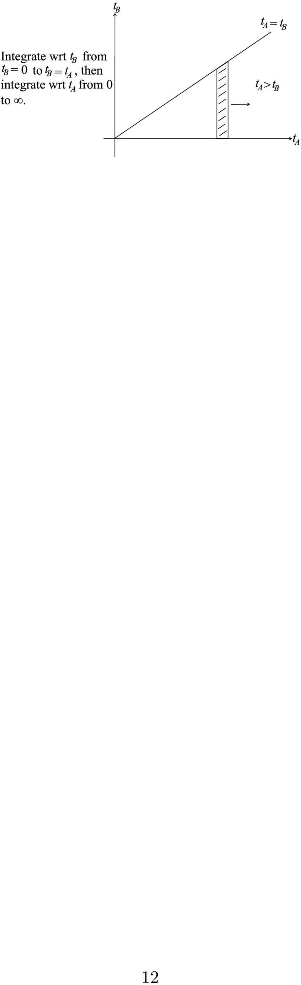
11 (ii) < y, Z z y z, z ; that is < y + z F Z (z) f Z (z) +z f XY (, dyd f XY (, + z) d π e z /4 e (+z) d π π e z /4 Eample Suppose two persons A and B come to two separate counters for service Let their service times be independent eponential random variables with parameters λ A and λ B, respectively Find the probability that B leaves before A? Solution Let T A and T B denote the continuous random service time of A and B, respectively Recall that the epected value of the service times are: E[T A ] and λ A E[T B ] That is, a higher value of λ implies a shorter average service time One λ B would epect P [T A > T B ] : P [T B > T A ] λ A : and together with P [T A > T B ] + P [T B > T A ], we obtain P [T A > T B ] λ B ; λ B λ A + λ B and P [T B > T A ] λ A λ A + λ B Justification:- Since T A and T B are independent eponential random variables, their joint density f TA,T B (t A, t B ) is given by f TA,T B (t A, t B ) dt A dt B P [t A < T A < t A + dt A, t B < T B < t B + dt B ] P [t A < T A < t A + dt A ]P [t B < T B < t B + dt B ] (λ A e λ At A dt A )(λ B e λ Bt B dt B ) P [T A > T B ] ta λ A λ B e λ At A e λ Bt B λ A e λ At A ( e λ Bt A ) dt A λ A e λ At A λ A λ A + λ B dt A λ B λ A + λ B dt B dt A λ A e (λ A+λ B )t A dt A

Solution Let T A and T B denote the continuous random service time of A and B, respectively Recall that the epected value of the service times are: E[T A ] and λ A E[T B ] That is, a higher value of

Math 431 An Introduction to Probability. Final Exam Solutions

Math 431 An Introduction to Probability. Final Exam Solutions Math 43 An Introduction to Probability Final Eam Solutions. A continuous random variable X has cdf a for 0, F () = for 0 <