DEVELOPMENT OF THE FORECAST PROPAGATION DATABASE FOR NOAA s SHORT-TERM INUNDATION FORECAST FOR TSUNAMIS (SIFT)

Transcription

1 NOAA Technical Memorandum OAR PMEL-139 DEVELOPMENT OF THE FORECAST PROPAGATION DATABASE FOR NOAA s SHORT-TERM INUNDATION FORECAST FOR TSUNAMIS (SIFT) Edison Gica 1,2 Mick C. Spillane 1,2 Vasily V. Titov 1,2 Christopher D. Chamberlin 1,2 Jean C. Newman 1,2 1 Joint Institute for the Study of the Atmosphere and Ocean (JISAO) University of Washington, Seattle, WA 2 Pacific Marine Environmental Laboratory Seattle, WA Pacific Marine Environmental Laboratory Seattle, WA March 2008 UNITED STATES DEPARTMENT OF COMMERCE Carlos M. Gutierrez Secretary NATIONAL OCEANIC AND ATMOSPHERIC ADMINISTRATION VADM Conrad C. Lautenbacher, Jr. Under Secretary for Oceans and Atmosphere/Administrator Office of Oceanic and Atmospheric Research Richard W. Spinrad Assistant Administrator

2 NOTICE from NOAA Mention of a commercial company or product does not constitute an endorsement by NOAA/OAR. Use of information from this publication concerning proprietary products or the tests of such products for publicity or advertising purposes is not authorized. Any opinions, findings, and conclusions or recommendations expressed in this material are those of the authors and do not necessarily reflect the views of the National Oceanic and Atmospheric Administration. Contribution No from NOAA/Pacific Marine Environmental Laboratory Also available from the National Technical Information Service (NTIS) ( ii

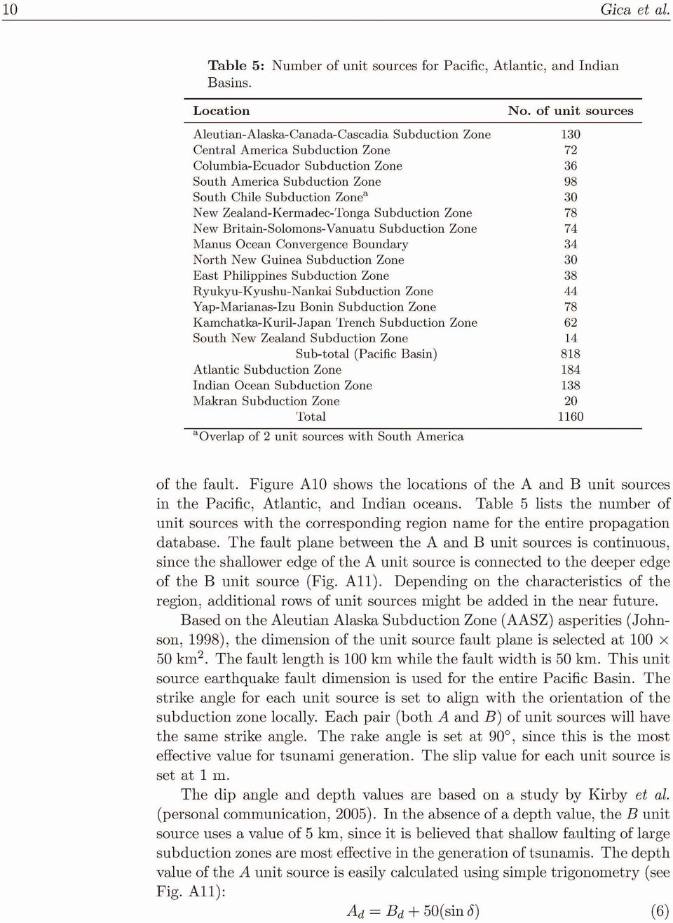
3 Contents Abstract 1 1 Background and Motive 1 2 Methodology Tsunami Generation Tsunami Propagation Pre-Defined Unit Sources Tsunami Model Input Parameters and Input/Output Data. 5 3 MOST Propagation Model Validation and Sensitivity Tests Model Validation Tsunami Sensitivity to Earthquake Source Parameters Sensitivity to epicenter Sensitivity to fault dimensions Sensitivity to dip and rake angles The Forecast Propagation Database Defining Unit Sources Forecast Propagation Database Validation Propagation Database Issues Initial Forecast Using M w Extent of Pacific Grid Domain and Total Run Time Propagation Database Forecast 14 7 Conclusions 15 8 Acknowledgments 16 9 References 17 Appendix A Figures 19 Appendix B Propagation Database Unit Source Information 39 List of Figures A1 Unit sources along the Aleutian Islands A2 Pacific map with the 1996 Andreanov epicenter and tsunami stations A3 Comparison of simulated tsunami wave with BPR s for the 1996 Andreanov tsunami iii

4 iv Contents A4 Bathymetry of the computational area, location of wave gages and earthquake epicenters for the sensitivity tests. 23 A5 Tsunami time series from different source locations A6 Directionality of generated tsunami A7 Tsunami time series comparison due to fault sensitivity. 26 A8 Tsunami time series comparison due to dip angle sensitivity 27 A9 Tsunami time series comparison due to slip angle sensitivity 27 A10a,b Unit sources for the Pacific Ocean A10c,d Unit sources for the Atlantic and Indian oceans A11 Sectional sketch of unit sources A and B A12 Propagation database forecast comparison with BPR records for the 1994 Kuril Island tsunami A13 Propagation database forecast comparison with DART records for the 2003 Rat Island tsunami A14 Propagation database forecast comparison with DART records for the 15 November 2006 Kuril tsunami A15 Location of offshore gages for comparison between MOST and SIFT results A16 Tsunami time series comparison between MOST and SIFT for different slip values with the same M w = A17 Propagating tsunami wave front comparison between two Pacific grids A18 Tsunami time series at south Australia and south Japan. 34 A19 Comparison of maximum tsunami wave amplitude distribution between two Pacific grids A20 Snapshot of tsunami forecast using websift A21 Forecasted tsunami first wave height at selected offshore A22 locations based on an M w = 7.5 in the Aleutian Islands.. 37 Snapshot of forecasted first tsunami wave and arrival time for Hilo Bay, Hawai i for sources from Ryukyus-Nankai, East Philippines and North New Guinea unit sources B1 Aleutians-Alaska-Canada Subduction Zones unit sources. 40 B2 Central America Subduction Zone unit sources B3 Ecuador-Columbia Subduction Zone unit sources B4 South America Subduction Zone unit sources B5 South Chile Subduction Zone unit sources B6 New Zealand-Kermadec-Tonga Subduction Zone unit sources B7 New Britain-Solomons-Vanuatu Subduction Zone unit sources B8 North New Guinea Subduction Zone unit sources B9 Manus Ocean Convergence Boundary unit sources B10 East Philippines Subduction Zone unit sources B11 Ryukyus-Kyushu-Nankai Subduction Zone unit sources.. 70 B12a Kamchatka-Yap-Mariana-Izu-Bonin unit sources, part B12b Kamchatka-Yap-Mariana-Izu-Bonin unit sources, part B13 Atlantic Subduction Zone unit sources B14 Indian Ocean Subduction Zone unit sources

5 Contents v B15 Makran Subduction Zone unit sources List of Tables Andreanov reference earthquake source parameters Epicenter variation for sensitivity analysis Fault dimension variation for sensitivity analysis Dip and rake angle variations for sensitivity analysis Number of unit sources for Pacific, Atlantic, and Indian Basins.. 10 B1 Aleutians-Alaska-Canada Subduction Zones unit sources parameters B2 Central America Subduction Zone unit sources parameters B3 Ecuador-Columbia Subduction Zone unit sources parameters B4 South America Subduction Zone unit sources parameters B5 South Chile Subduction Zone unit sources parameters B6 B7 New Zealand-Kermadec-Tonga Subduction Zone unit sources parameters New Britain-Solomons-Vanuatu Subduction Zone unit sources parameters B8 North New Guinea Subduction Zone unit sources parameters B9 Manus Ocean Convergence Boundary unit sources parameters.. 67 B10 East Philippines Subduction Zone unit sources parameters B11 Ryukyus-Kyushu-Nankai Subduction Zone unit sources parameters. 71 B12 Kamchatka-Yap-Mariana-Izu-Bonin unit sources parameters B13 Atlantic Subduction Zone unit sources parameters B14 Indian Ocean Subduction Zone unit sources parameters B15 Makran Subduction Zone unit sources parameters

6

7 Development of the forecast propagation database for NOAA s Short-term Inundation Forecast for Tsunamis (SIFT) E. Gica 1,2, M.C. Spillane 1,2, V.V. Titov 1,2, C.D. Chamberlin 1,2, and J.C. Newman 1,2 Abstract. The NOAA Center for Tsunami Research (NCTR) is developing an operational tool that provides quick and accurate tsunami forecasts known as Short-term Inundation Forecast for Tsunamis (SIFT). The SIFT system uses Deep-ocean Assessment and Reporting of Tsunamis (DART ), data inversion techniques, tsunami propagation estimates, and site specific inundation forecasts. SIFT is an efficient and accurate operational tool that can provide offshore forecasts of tsunami time series quickly at any specified site. Providing a quick tsunami forecast is possible with the aid of the forecast propagation database which is set up by pre-computing earthquake events using unit sources along the known and potential earthquake zones in the Pacific, Atlantic, and Indian oceans. Currently 1160 unit sources have been simulated to provide Pacific, Atlantic, and Indian ocean coverage. Tsunami generation and propagation is simulated using the MOST propagation code. Exploiting the linearity of the generation/propagation dynamics, the propagation database can simulate arbitrary earthquake scenarios using combination unit sources that can accurately reproduce tsunami time series as validated with ten real tsunami events since Background and Motive NOAA tsunami warning centers and officials at other agencies are in urgent need of an operational tool that can provide quick and accurate tsunami forecasts to guide their decisions for issuing tsunami warnings. Forecasting tsunami impacts for any coastal area right after a tsunamigenic event is a tremendous achievement and is very useful to the tsunami warning centers and hazard mitigation managers. The NOAA Center for Tsunami Research (NCTR) is developing a tsunami forecast system known as Short-term Inundation Forecast for Tsunamis (SIFT) that uses data inversion technique and site-specific inundation forecasts (referred to as Standby Inundation Models or SIMs). Data inversion will combine real-time DART data (recordings from the NTHMP tsunameters: González et al., 2005) with pre-computed scenarios (forecast propagation database) while SIMs will provide forecasts for coastal areas. The forecast propagation database is set up by pre-computing earthquake events. Developing the offshore forecast database is possible because of the linearity of the generation/propagation dynamics whereby base scenarios can be combined linearly to relate the earthquake parameters to the generated tsunami s wave height, period, and directionality off the coast. The results of the propagation scenario also serve as input for the SIMs that numerically predict the tsunami wave height, current speeds, and inundation extent of a specific coastal area of interest. Fast real-time forecast modeling of tsunami waves is complicated by the fact that current technology cannot provide all the earthquake parameters needed for simulation immediately after an earthquake event. NCTR s data 1 NOAA, Pacific Marine Environmental Laboratory, Seattle, WA , USA 2 Joint Institute for the Study of the Ocean and Atmosphere (JISAO), Box , University of Washington, Seattle, WA , USA

8 2 Gica et al. inversion technique is a solution for this problem. Forecast is done using pre-defined typical earthquake parameters (i.e., dip and rake-angles, slip, depth of source), which are adjusted to the epicenter and moment magnitude, M w, obtained after an event. Once the DART buoys pick up the tsunami waves, inversion is done to refine the tsunami source region. The propagation database has been validated with ten real tsunami events since 2003 and is thoroughly tested for accuracy, reasonableness of results, and error sensitivity. It should be noted that the variability of an arbitrary tsunami generation mechanism is too large to store in a database. Doing so would require infinitely large storage. The solution is to select a limited number of scenarios that would represent all possible events with accountable accuracy. This can be done by sensitivity tests to determine which earthquake parameters provide the most variability for generated tsunami waves. The methodologies, theories, and sensitivity tests used in the development of the pre-defined, pre-computed sources validation with historical and real-time events, practical use, and sensitivity of the propagation database itself are discussed in this report. 2. Methodology SIFT uses a two-step process: (1) data inversion, which combines real-time seismic and tsunami data with the pre-computed scenarios (forecast propagation database); (2) the site-specific inundation forecast using SIMs. This section describes the theories and methodologies used in the development of the propagation database. 2.1 Tsunami Generation The initial tsunami generation model follows a commonly used method whereby the initial sea surface displacement follows that of the final vertical displacement of the ocean bottom due to an earthquake. An elastic deformation (Okada, 1985) source model is applied to determine the shape of the earthquake s vertical displacement, which assumes the rupture of a single rectangular fault plane. The earthquake parameters required for the model are the fault s length, L, and width, W, location or epicenter, fault s orientation or strike angle, θ, dip angle, δ, rakeangle,λ, average slip, u o, and depth of source, h. Calculation of the earthquake s seismic moment uses the following equation: M o = μu o LW (1) where the earth s rigidity, μ, is assumed to be dynes/cm 2, u o, L and W in cm.

9 Development of forecast propagation database for NOAA s SIFT 3 The moment magnitude, M w, can then be computed by using the following formula: M w = 2 3 log (M o) 10.7 (2) An earthquake source could contain multiple sub-faults with very complex slip distributions. Obtaining all details of an earthquake source could take months of analysis using high-quality data. Okada s (1985) source model is very simple; however, estimates of earthquake parameters (i.e., slip, depth of source, epicenter, and moment magnitude, M w ) are readily available after an earthquake event, making it very useful for tsunami mitigation. The earthquake parameters then serve as input to the MOST deformation code, which uses the Okada (1985) source model, to generate the earthquake source deformation, which will determine the initial tsunami s characteristics. This becomes one of the input files for the MOST propagation code. 2.2 Tsunami Propagation After the initial tsunami wave is generated by an earthquake, the waves will radiate away from the source and propagate in the open ocean. Tsunami waves can propagate across entire ocean basins, and since it covers a very large area, the curvature of the earth is taken into account. The MOST propagation code uses the non-linear shallow water equation in spherical coordinates with Coriolis force and a numerical dispersion scheme to take into account the different propagation wave speeds with different frequencies. The equations, shown below, are numerically solved using a splitting method (Titov, 1997): h t + (uh) λ +(vh cos φ) =0 R cos φ (3) u t + uu λ R cos φ + vu φ R + gh λ uv tan ϕ = gd λ R cos φ R R cos φ C fu u + fv d (4) v t + uv λ R cos φ + vv φ R + gh φ R + u2 tan ϕ = gd φ R R C fv u fu d (5) where: λ = longitude φ = latitude h = h (λ, φ, t)+d (λ, φ, t) h (λ, φ, t) = amplitude d (λ, φ, t) = undisturbed water depth u (λ, φ, t) = depth-averaged velocity in longitude direction v (λ, φ, t) = depth-averaged velocity in latitude direction g =gravity R =radiusoftheearth f =2ω sin φ, Coriolis parameter C f = gn 2 /h 1/3,nis Manning coefficient

10 4 Gica et al. The propagation database covers Pacific, Atlantic, and Indian oceans. The Pacific Ocean bathymetry for the numerical simulation is based on Smith and Sandwell (1994) 2 arc-minute data. The Atlantic Ocean bathymetry is derived from several sources. Higher resolution data are generally available near the coastal areas. Sources for the Atlantic are from Smith and Sandwell (1994) 2 arc-minute data, General Bathymetric Chart of the Oceans (GEBCO), National Ocean Service, National Tsunami Warning and Mitigation Program, National Geospatial-Intelligence Agency (NGA), Scripps Institution of Oceanography, University of Rhode Island, Woods Hole Oceanographic Institution, Lamont-Doherty Earth Observatory, U.S. Geological Survey, and Center for Coastal and Ocean Mapping/Joint Hydrographic Center (CCOM/JHC) of the University of New Hampshire, Instituto Nacional de Estadística Geografía e Informática (INEGI), NOAA s Office of Ocean Resources Conservation and Assessment, Strategic Environmental Assessments (SEA) Division, Joint Airborne LIDAR Bathymetry Technical Center of Expertise-JALBTCX (U.S. Army Corps of Engineers) and International surveys. The Indian Ocean bathymetry is also derived from several sources: data are from SRTM30, coastal and ridge multibeam (Scripps Institution of Oceanography, 2004), University of Southern California Tsunami Research Center (Greeninfo Network), and National Geospatial-Intelligence Agency (NGA). Although high-resolution bathymetry data is available for the Pacific, Atlantic, and Indian oceans, the bathymetry is re-gridded to 4 arc-minute, which is used in the simulation. The output data is reduced in size by saving a coarser grid of 16 arc-minutes resolution and 1 minute in time. There are currently two Pacific grid domains. The regular Pacific grid covers 62 Nto50 S and 120 E to 292 E and the extended one covers 62 N to 74 S and 120 E to 292 E, which extends 24 further south as compared to the regular Pacific grid. The grid extent for the Atlantic is from 105 W to 20 Eand72 Nto72 S, while the Indian Ocean covers 0 Eto60 Eand 32 Nto70 S. The time step used in the simulation depends on the grid that is being used since it has to follow the CFL condition. For the regular Pacific grid, the CFL condition requires a time step of 15 seconds, while the extended Pacific requires a time step of 12 seconds. The Atlantic Ocean uses a time step of 10 seconds, while the Indian Ocean uses 12 seconds as required by the CFL condition. Comparison of the two Pacific grid domains was conducted and is explained in section 5.2. Tests are currently being done to develop a global grid containing all the unit sources in the Pacific, Atlantic, and Indian oceans. 2.3 Pre-Defined Unit Sources The main objective of the pre-computed tsunami database is to be able to provide offshore forecasts of tsunami amplitudes and other wave parameters quickly without having to run simulations right after a tsunamigenic event. The goal is to define an earthquake source region such that a finite combination of those could closely reproduce the tsunami time series

11 Development of forecast propagation database for NOAA s SIFT 5 of the actual event. This is feasible because of the linearity of the generation/propagation dynamics. Each pre-defined earthquake source is referred to as a unit source. Each unit source has a fault length of 100 km, fault width of 50 km, and a slip value of 1 m, generating an equivalent moment magnitude, M w,of7.5. Two rows of unit sources are set up, one for the shallower region and one for the deeper region. Additional rows may be possible depending on the characteristics of the region. These unit sources are located along the known fault zones for the entire Pacific Basin, Caribbean for the Atlantic region and Indian Ocean. Figure A1 shows how the unit sources will be set up. 2.4 Tsunami Model Input Parameters and Input/Output Data Earthquake parameters: the generation of the initial tsunami wave requires the input of earthquake parameters: epicenter (longitude and latitude), fault length, fault width, dip, rake, and strike angles, slip value, and depth. Bathymetry data: A 4 arc-minute grid resolution (see section 2.2); land is specified as a negative value, water as positive. Three output files are generated in netcdf format for the following variables: Simulated tsunami wave height, ha Simulated tsunami velocity in x-direction, u Simulated tsunami velocity in y-direction, v 3. MOST Propagation Model Validation and Sensitivity Tests This section briefly discusses the validation of the MOST propagation code with a real tsunami event; other validations (i.e., lab experiments, etc.) are described in Titov (1997). Sensitivity tests of the tsunami time series to earthquake source parameters for far-field tsunamis are also investigated. 3.1 Model Validation The first validation of the global propagation (i.e., MOST) code was done with the 10 June 1996 Andreanov tsunami (Titov and González, 1997). Several deep ocean Bottom Pressure Recorder (BPR) records of the event were compared with the simulation for the 10 June 1996 Andreanov tsunami. The estimated seismic moment, M o,of N m was obtained from the Harvard solution; aftershock distribution estimated the source region to be 140 km long and 70 km wide. Assuming a shear modulus, μ, of

12 6 Gica et al. N m, the average slip, u o, was estimated to be 2 m (using Equations 1 and 2). Using a single-fault mechanism for the source region, a comparison was made between the simulated tsunami wave time series with that of the data obtained by the BPRs from the actual event. The location of the Andreanov earthquake source and the BPRs are shown in Fig. A2. The grid domain for the simulation covers the North Pacific region (15 Nto65 N and 180 W to 120 W) with 4 arc-minute bathymetry data from Smith and Sandwell (1994). Comparison was made at five BPR stations and the results showed that the MOST propagation code was able to reproduce with sufficient accuracy the dominant deep-ocean wave form for the Andreanov tsunami (Fig. A3). 3.2 Tsunami Sensitivity to Earthquake Source Parameters A commonly used method to define the initial tsunami surface is to apply the same displacement as the vertical deformation of the ocean bottom due to the earthquake. This makes the initial sea surface displacement a function of the earthquake parameters, namely: fault length, fault width, dip, rake, and strike angles, epicenter, depth, and slip values. The question is, would the tsunami time series be sensitive to the details of the source? Earthquake parameters available right after an earthquake are preliminary and could be inaccurate. Determining which earthquake source parameters would affect the far-field tsunami time series will show the sensitivity of the tsunami time series to seismic source details. Sensitivity to the earthquake parameters was studied using the 10 June 1996 Andreanov Island tsunami event, since the MOST generation and propagation model showed favorable comparison with the deep-ocean data from the BPRs (Titov and González, 1997), as shown in Fig. A3. The sensitivity tests (Titov et al., 1999) were conducted to determine if deviation of the earthquake source parameters would produce an unacceptable model-data comparison and is discussed here. Certain earthquake parameters are geographically constrained. The focal depth was set to 5 km and the strike angle was aligned with the Aleutian trench, which tends to be characteristic of most large underthrust earthquakes in the Alaskan-Aleutian subduction zone (AASZ). The last important constraint was setting the seismic moment, M o,to N m, as estimated for the Andreanov earthquake for all the model sources. With those constraints in place, earthquake source parameters such as epicenter, fault length, fault width, dip and rake angles, were then varied. The mean slip value, u o, is determined from Equation 1. Reference values are listed in Table 1. Numerical stations to compare the simulated tsunami time series are shown in Fig. A4. Numerical gage 1 is located near Hawai i at a depth of 4747 m, while gage 2 is between Hawai i and the AASZ at a depth of 5910 m. Both numerical gages 1 and 2 are deep enough to ensure linearity of the wave dynamics. Numerical gage 3 is located on Axial Seamount at

13 Development of forecast propagation database for NOAA s SIFT 7 Table 1: 1996 Andreanov reference earthquake source parameters. Earthquake Source Parameter* Value Epicenter (latitude, longitude) 51.2 N, E Fault Length (km) 140 Fault Width (km) 70 Dip angle (degrees) 20 Rake angle (degrees) 108 *Source: Titov and González (1997). a depth of 1550 m. The bottom pressure recorder (BPRs) locations are markedasnos.4to7. Using the reference earthquake source parameter (Table 1), variations for the earthquake s epicenter, fault area, and dip and rake angles are simulated and compared. Table 2 lists the epicenter variation, while Tables 3 and 4 list the variation for fault dimensions and dip- and rake angles, respectively. It can be seen in Table 3 that the slip values change as the fault dimension is varied. This has been done to preserve the earthquake s magnitude. It should be noted that the rupture size of an earthquake right after the event is not immediately available. High-quality data with months or even years of analysis are required to get a reasonable estimate. Several empirical formulas that relate the fault s size and rupture extent to the earthquake magnitude are currently used for quick evaluation of real-time tsunami assessment Sensitivity to epicenter The characteristics of the tsunami waves generated from an earthquake source vary according to where the source is located. Its sensitivity is tested by varying the epicenter at seven different locations (Table 2). The strike angle values are adjusted to align with the Aleutian trench. To have a better view of the comparison, the timescale has been shifted to match that of the Andreanov tsunami arrival time. Comparison at Gage 1 of the simulated results showed that the leading tsunami wave height is similar for almost all source locations, with the exception of source G (see Fig. A5 and Table 2), which is about half that of the other sources. The leading tsunami wave height at Gage 2 drops as the source location moves eastward. Source A is 2.7 times more than source G at Gage 2. This trend is reversed at Gage 3. Source G is 5.5 times that at Source A, which had the smallest amplitude. Cylindrical spreading causes the tsunami waves to decrease in height as they move further away from the generating source. Also, tsunami energy tends to be directional. The majority of the tsunami energy is propagating out at a right angle from the source region. The directionality of the tsunami beam is shown in Fig. A6, representing sources A and G with contours of maximum computed amplitudes. It can be seen that as the tsunami wave propagates off-shore, the amplitude is much higher in the direction which is perpendicular to the trench or the fault. The further away a coastal area is from the main beam the smaller

14 8 Gica et al. Sources Table 2: Epicenter variation for sensitivity analysis*. Lon Lat Length Width Strike Dip Rake Depth Slip N E (km) (km) (deg) (deg) (deg) (km) (m) A B C D E F G *Source: Titov et al. (1999). Sources Table 3: Fault dimension variation for sensitivity analysis*. Lon Lat Length Width Strike Dip Rake Depth Slip N E (km) (km) (deg) (deg) (deg) (km) (m) H I J K L M *Source: Titov et al. (1999). Sources Table 4: Dip and rake angle variations for sensitivity analysis*. Lon Lat Length Width Strike Dip Rake Depth Slip N E (km) (km) (deg) (deg) (deg) (km) (m) N O P Q R S T *Source: Titov et al. (1999). the tsunami amplitude will be. This is one factor in why the tsunami wave amplitude at Gage 1 for source G is much smaller than the other sources (see Fig. A6). Another factor is the bathymetry profile around the area of source G. The Gulf of Alaska has a series of seamounts that can affect the tsunami propagation characteristics, unlike other sources that are not affected by similar bathymetric features Sensitivity to fault dimensions Sensitivity to fault dimensions was tested by varying the fault area as listed in Table 3. Comparison was made by maintaining the earthquake seismic moment (M o = N m); thus the slip values were adjusted according

15 Development of forecast propagation database for NOAA s SIFT 9 to Equations 1 and 2. Results showed that even with a three-fold increase in the slip value (sources L and M in Table 3, with the corresponding fault dimensions) the leading tsunami wave height was within 25% of the maximum at Gages 1 and 2 (Fig. A7). The gages near the continental coast (Gages 3 and 4) showed more difference for the leading tsunami waves, but are within 50% of the maximum at these gages Sensitivity to dip and rake angles A small variation of the dip and rake angles was tested for sensitivity of the tsunami wave heights. The epicenter of the source region is based on the Andreanov earthquake as shown in Table 5. The dip angle was tested between 10 and 20 with a 5 increment. A 10 to 20 range is typical of the subduction earthquakes in the AASZ. Simulated results show that the leading tsunami waves (comparison at gages 1 and 2) increased by 30%, but the wave period and profile of the first wave were very similar for all the dip values (Fig. A8). The variation of the rake angle ranges from a pure dip-slip mechanism (rake = 90 ) to a 50% strike-slip mechanism with a rake value of 135. Comparing the simulated results at Gages 1 and 2, the tsunami wave height did not show a significant variation (Fig. A9). The leading tsunami wave height for a strike-slip component is 20% less that a pure dip-slip one. The earthquake source parameters that are available after an earthquake event are preliminary. Real-time data inversion of the tsunami signal obtained by the Deep-ocean Assessment and Reporting of Tsunamis (DART ) buoys will refine the tsunami source. However, the results of the sensitivity tests establish the fact that the far-field tsunami time series is only sensitive to the earthquake s epicenter and magnitude, which can be obtained with considerable accuracy. Variations of the other source parameters tested (i.e., fault dimensions, dip and rake angles) do not change the tsunami signal significantly. 4. The Forecast Propagation Database This section describes how the unit source was defined, the regions it is applied to, and its validation with two real tsunami events. 4.1 Defining Unit Sources The earthquake source region selected for the propagation database is based on a typical subduction mechanism with a moment magnitude (M w )of7.5. This is referred to as a unit source. These unit sources are arranged side-byside along the subduction zones (trench axis) or earthquake source regions forming a continuous line of faults, and are referred to as B unit sources. A second set of unit sources is placed in parallel with the B unit sources, referred to as the A unit sources, which are located on the deeper part

16

17 Development of forecast propagation database for NOAA s SIFT 11 where: A d =depthofa unit source B d =depthofb unit source δ = dip angle of B unit source If new data are available for depth value, those B unit sources that have a depth value of 5 km will then be updated, together with the A unit sources, and re-simulated. The propagation runs do not include inundation and a vertical wall is placed at 20 m water depth. Simulation runs are done on a 4 arc-minute resolution but saved on a 16 arc-minute resolution to minimize file size. The simulation time step is 15 seconds for the regular Pacific grid (120 Eto 292 Eand62 Nto50 S), 12 seconds for the extended Pacific grid (120 Eto 292 Eand62 Nto74 S), 10 seconds for the Atlantic grid (105 Wto20 E and 72 Nto72 S) and 12 seconds for the Indian ocean grid (0 Eto60 E and 32 Nto70 S). The time steps are based on CFL stability criteria. Time step resolution for the output file is 1 minute. The total simulation time is 24 hours, with the exception of the East Philippines and North New Guinea sources, which were simulated for 30 hours. Discussions on the two different Pacific grids and the two simulation run times used in the simulations are in Section Forecast Propagation Database Validation The main idea of the unit sources was that a finite combination would reproduce as close as possible to the actual tsunami time series. Preliminary forecast of the ocean wide tsunami time series are quickly produced by combining unit sources once the initial earthquake parameters (epicenter and magnitude) are obtained from the Tsunami Warning Center (TWC). Once the DART buoy(s) receives the actual tsunami wave, inversion is then performed to adjust the slip distribution of the selected unit sources or add unit sources as needed. This methodology was verified with ten real tsunami events since 2003 and a few are presented in this report, namely: the 4 October 1994 Kuril Island (Yeh et al., 1995), the 17 November 2003 Rat Island (Titov et al., 2005), and 15 November 2006 Kuril tsunamis. For the 4 October 1994 Kuril Island tsunami, inversion was done from five DART buoy records and the forecast showed good comparison as seen in Fig. A12. When the closest DART buoy (Sta D171) recorded the actual tsunami waves of the 17 November 2003 Rat Island tsunami, adjustments were made and the forecast even had an excellent comparison with the tsunami records at other locations (Fig. A13). In fact, the forecast gave a better estimate of the earthquake magnitude (M w = ) as confirmed later by USGS seismic analysis (M w = 7.8) (NEIC, 2003), where the initial earthquake magnitude was M s = 7.5 as provided by West Coast/Alaska TWC. It took only 1 hour 20 minutes after the earthquake to provide an accurate forecast. Combining the propagation database and real-time DART data from the tsunameters, tsunami waves were predicted well before the actual waves

18 12 Gica et al. hit the coastlines. This again was demonstrated for the 15 November 2006 Kuril tsunamis. Figure A14 shows the good comparison between the DART time series and that based on inversion. Although not part of the TWC operation, the validations of the propagation database with real events show that sets of pre-computed unit sources can be combined to produce tsunami scenarios that would closely match the recorded data from the tsunameters from real tsunamigenic events. The methodology is not only accurate but also very efficient, considering that an accurate forecast is provided a few hours after a tsunamigenic event. 5. Propagation Database Issues With the unit source defined, simulation was done for the entire Pacific, Atlantic, and Indian oceans and stored in a database. Validation with ten real tsunami events since 2003 demonstrated that the forecast propagation database methodology can reproduce the tsunami signal of the actual event. This section investigates several non-critical issues, proposed solutions, and aspects of using the database itself for forecasts. 5.1 Initial Forecast Using M w Each unit source has been simulated and the tsunami wave height, ha, andu and v, velocity components stored in a database. Tsunami scenarios can then be constructed from a combination of unit sources by exploiting the linearity of the generation/propagation dynamics to match closely the actual tsunami wave amplitude recorded by the DART buoys. Initial forecasts will require the input of an earthquake magnitude and location. Once the tsunami wave has been detected by the DART buoys, then the initial model predictions from the propagation database will be adjusted to provide a more accurate prediction. The unit sources are based on an earthquake magnitude, M w,of7.5. Using the linearity dynamics of generation and propagation, the tsunami amplitudes for an M w > 7.5 are quickly estimated by multiplying numerical values in the database. These numerical values are obtained using Equations 1 and 2. For example, if we consider one unit source with an M w =8.5, with only u o as the unknown, using Equations 1 and 2 would yield an average slip value, u o, of m. The value of m will be the multiplying factor for the unit source database. However, an average slip value of 26.6 m to 37.4 m can still produce an M w =8.5 when using Equations 1 and 2. Unit source B11 in the East Philippines was chosen arbitrarily to investigate by how much the tsunami amplitude would differ. Figure A15 shows the comparison at three deep ocean regions: near the source, Hawai i, and South America regions. An average slip of m yields a tsunami wave time series that is ±20% from the two extremes (i.e., 26.6 m and 37.4 m), as seen in Fig. A16.

19 Development of forecast propagation database for NOAA s SIFT 13 The ±20% variation in the forecasted tsunami wave time series is not an error range produced by the MOST propagation code. This variation is inherent in the equations for calculating the M w (Equation 2) due to rounding off. Data inversion will provide a more accurate forecast with the adjusted tsunami source. Care must be taken when only seismic data is used to obtain the tsunami propagation forecast. 5.2 Extent of Pacific Grid Domain and Total Run Time As the number of unit sources expand in the database, the need for possibly extending the previous Pacific grid (which covers 120 E to 292 Eand62 N to 50 S) became apparent, especially for the unit sources south of the South America region, and due to the presence of the great circle routes of tsunami propagation in the Antarctic. Using the propagation database, unit source A37 in the South America Subduction Zone was selected to determine the difference of the tsunami time series between using the regular Pacific grid and the extended Pacific grid (which covers 120 E to 292 Eand62 Nto 70 S) at a station south of Australia (130 E, 40 S; see Fig. A17). As the propagating tsunami moves toward Australia, it clearly show the difference between the Pacific grid that stops at 50 Sfromthatat74 S (Fig. A17). The open boundary at 50 S prevents the tsunami waves from traveling the great circle in that region, however; the additional 24 to the south puts this into the path of the propagating tsunami waves. The leading tsunami wave on the extended Pacific grid does not exist on the regular Pacific grid at time step 791 (Fig. A17). A plot of the tsunami time series for the regular Pacific grid shows that the entire tsunami time series of the previous grid is one order of magnitude smaller than the first wave alone using the extended grid (Fig. A18). A plot of the maximum wave height distribution (Fig. A19) shows that much higher maximum wave heights cover the entire northern coast and almost the entire eastern coast of New Zealand when using the extended Pacific grid as compared with the regular Pacific grid. Another aspect investigated was the total number of hours required for each unit source simulation in the propagation database. The majority of the unit sources cover 24 hours of tsunami time series; a few (North New Guinea and East Philippines) cover 30 hours, since the leading tsunami wave would barely reach central South America. Using the same unit source (A37 in the South America Subduction Zone), the time series was checked near Japan (130 E, 30 N, Fig. A17). Figure A19 shows that the first wave was not completely simulated at this location, indicating that 24 hours or 30 hours of tsunami time series might not be enough to be able to capture the maximum tsunami wave. Recognizing these two issues is crucial, although not critical, for the propagation database, especially since it is an offshore forecast tool, it should be noted that the 22 May 1960 Chile tsunami did reach Japan. These issues will be resolved by determining the maximum grid extent to be used for the Pacific Ocean, as well as the total run time, by conducting tests. Once

20 14 Gica et al. it has been determined, the propagation database will then be updated. It should be noted that the current issues do not affect the current propagation database, because there are sufficient tsunami time series for the Alaskan- Aleutian, U.S. West coast, and Hawai i regions from all the unit sources. 6. Propagation Database Forecast The output of the propagation database not only serves as input for the SIMs, but in itself can be used for offshore tsunami forecasts. As previously shown (see Section 4.2), a combination of unit sources can reproduce tsunami scenarios quickly, showing the offshore tsunami wave characteristics for the Pacific, Atlantic, or Indian ocean domains and offshore forecast for specific locations. Obtaining the arrival time, distribution of the first tsunami wave height, maximum wave height, and tsunami beam quickly are invaluable information needed for hazard mitigation. A sample snapshot (Fig. A20) shows the first wave and maximum wave forecast in websift using a single unit source located at the Aleutians with an earthquake M w of 7.5. Plotting the forecast tsunami first wave height at selected offshore points in Pacific coasts can also be provided (Fig. A21). Information obtained can immediately provide assessments on which areas will primarily be affected by the simulated tsunami waves. It is also possible to include arrival time. This can serve as a guideline for prioritizing the inundation forecast of coastal areas using the SIMs. The propagation database can also be used to determine the tsunami risk to a specific coastal area and which source region would provide the most threat. For illustrative purposes, using only one unit source, several earthquake scenarios with M w values of 7.5, 8.0, 8.5, and 9.0 were generated and the tsunami s first wave height was determined for Hilo Bay, Hawai i. A snapshot for sources from Ryukyus-Nankai, East Philippines, and North New Guinea subduction zones are shown in Fig. A22. Comparing the three subduction zones, the East Philippines source especially, the mid-section shows more of a threat for Hilo as compared with Ryukyus-Nankai and North New Guinea sources. It can also be seen that although the tsunami waves arrive close to 11 hours after the generation, the first wave from East Philippines unit source B11 is the highest compared to Ryukyus-Nankai and North New Guinea sources, which arrived at a much earlier time. The forecast capability of the propagation database provides invaluable information to the TWC personnel. The propagation database forecast results can provide guidelines on prioritizing which specific coastal site needs immediate attention during a real tsunami event.

21 Development of forecast propagation database for NOAA s SIFT Conclusions The operational tool that will provide quick and accurate tsunami forecasts, developed by the NCTR, has been tested to be efficient and accurate. The method referred to as Short-term Inundation Forecast for Tsunamis (SIFT) uses data inversion technique and SIMs. One of the key components of this system is the pre-computed earthquake scenarios (forecast propagation database). The pre-computed tsunami scenarios are simulated from a unit source with an earthquake moment magnitude, M w,of7.5. Unitsources have been established in the known and potential earthquake regions with a total of 1160 sources for the Pacific, Atlantic, and Indian oceans, (including Makran sources, not shown in Fig. A10). Exploiting the linearity of the generation/propagation, a combination of these unit sources can simulate tsunami scenarios. Tests conducted with real-time tsunami events show that, with data inversion, it can closely match the actual tsunami time series. Other than its accuracy, prediction of the tsunami wave signal took just 1.5 hours after the 17 November 2003 Rat Island earthquake event several hours before the actual waves hit the coastlines of Hawai i, Alaska, and the U.S. West Coast. Accuracy of the source parameters might come into question; however, sensitivity tests conducted show that only the earthquake s epicenter and magnitude would cause a significant variation in the far-field tsunami time series using the MOST code. Also, data inversion of the tsunami signals obtained from the DART buoys will refine the tsunami source. A few non-critical issues on the use of the propagation database for preliminary forecasts were investigated. Several values of slip can produce the same earthquake seismic magnitude, M w, when using Equations 1 and 2, due to a one-decimal-place rounding. However, if slip value is to be obtained directly from Equations 1 and 2 with known fault dimensions and earth s rigidity, μ, the resulting slip value is roughly 1.4% below the average of the lowest and highest possible slip values producing the same M w. This value is used as a multiplying factor for the propagation database for M w > 7.5. Tests conducted show that the tsunami time series of the forecast propagation database is ±20% that of the lowest and highest possible slip values under the same M w. This will not be an issue when data inversion is used, but should be kept in mind if a real-time tsunami signal is not available. The other non-critical issues were the extent of the Pacific domain and the total simulation hours in the propagation database. Test results show that the presence of the great circle in the Antarctic could potentially pose a tsunami threat to South Australia as opposed to no threat, especially from sources in South America when the simulation domain does not include the great circle. Total simulation time was either 24 hours or 30 hours, since the tsunami signal for some sources (e.g., East Philippines and North New Guinea) would barely reach certain areas on the other side of the Pacific. The

22 16 Gica et al. reason for limiting simulation to 30 hours is that the tsunami signal would reach most of the regions on the other side of the Pacific basin, and would also generate a smaller output file size. However, it has been recognized that the non-critical issues of the extent of the Pacific domain and total simulation hours in the propagation database might pose a problem in the future. These issues are currently being resolved by conducting tests on what the maximum extent of the Pacific domain should be, including the total simulation hours, so as to obtain sufficient tsunami time series on either side of the Pacific basin. The output of the forecast propagation database not only serves as input for the SIMs that numerically predict the tsunami wave height, current speeds, and inundation extent of a specific coastal area of interest, but can be used to forecast offshore tsunami wave heights at any specified location in the Pacific, Atlantic, and Indian oceans. Regional and site-specific first and maximum wave height and arrival time can be plotted quickly. It is also possible to plot the offshore wave height distribution for the entire Pacific, Atlantic, and Indian ocean coasts. This will graphically show the coastal areas that have a higher risk of tsunami threat during an actual event. 8. Acknowledgments This publication is contribution 2937 from NOAA/Pacific Marine Environmental Laboratory and funded by the Joint Institute for the Study of the Atmosphere and Ocean (JISAO) at the University of Washington under NOAA Cooperative Agreement No. NA17RJ1232, JISAO contribution The authors would also like to thank R.L. Whitney for comments and edits, and Christopher Moore for providing the images for Figure A10.

23 Development of forecast propagation database for NOAA s SIFT References González, F.I., E.N. Bernard, C. Meinig, M. Eble, H.O. Mofjeld, and S. Stalin (2005): The NTHMP tsunameter network. Nat. Hazards, 35 (1), Special Issue, U.S. National Tsunami Hazard Mitigation Program, Johnson, J. (1998): Heterogeneous coupling along the Alaskan-Aleutians as inferred from tsunami, seismic, and geodetic inversions. Adv. Geophys., 39, 1 116, (R. Dmowska, ed.), Academic Press. Kirby, S., E. Geist, W.H.K. Lee, D. Scholl, and R. Blakely (2005): Tsunami source characterization for Western Pacific subduction zone: A preliminary report. USGS Tsunami Subduction Zone Working Group (personal communication). NEIC (2003): Poster of the Rat Islands, Alaska earthquake of 17 November 2003 Magnitude Okada, Y. (1985): Surface deformation due to shear and tensile faults in a halfspace. Bull. Seismol. Soc. Am., 75, Scripps Institution of Oceanography (2004): ucsd.edu/www_html/srtm30_plus.html. Satellite geodesy. Smith, W.H.F., and D.T. Sandwell (1994): Bathymetric prediction from dense satellite altimetry and sparse shipboard bathymetry. J. Geophys. Res., 99, 21,803 21,824. Titov, V.V. (1997): Numerical modeling of long wave run-up. Ph.D. thesis, University of Southern California, Los Angeles, California, 141 pp. Titov, V.V., and F.I. González (1997): Implementation and testing of the Method of Splitting Tsunami (MOST) model. NOAA Tech. Memo. ERL PMEL-112 (PB ), NOAA/Pacific Marine Environmental Laboratory, Seattle, WA, 11 pp. Titov, V.V., F.I. González, E.N. Bernard, M. Eble, H.O. Mofjeld, J. Newman, and A.J. Venturato (2005): Real-time tsunami forecasting: Challenges and solutions. Nat. Hazards, 35, Titov, V.V., H.O. Mofjeld, F.I. González, and J.C. Newman (1999): Offshore forecasting of Alaska-Aleutian Subduction Zone tsunamis in Hawaii. NOAA Tech. Memo. ERL PMEL-114, (NTIS PB ), NOAA/Pacific Marine Environmental Laboratory, Seattle, WA, 22 pp. Yeh, H., V.V. Titov, V. Gusiakov, E. Pelinovsky, V. Khramushin, and V. Kaistrenko (1995): The 1994 Shikotan earthquake tsunami. Pure Appl. Geophys., 144 (3/4),

24

25 Development of forecast propagation database for NOAA s SIFT 19 Appendix A. Figures

26 20 Gica et al. (a) aerial view (b) side aerial view Figure A1: Unit sources along the Aleutian Islands.

27 Development of forecast propagation database for NOAA s SIFT o N 55 o N 45 o N 35 o N 25 o N 15 o N 5 o N 5 o S 15 o S , , , , , , , , , , , , , o S 152, o S o E 130 o o o E 145 E 160 E 175 o E 170 o W 155 o W 140 o W 125 o W 110 o W 95 o W 80 o W 65W o Figure A2: Pacific map with the 1996 Andreanov epicenter (star) and tsunami stations. Deep ocean BPR data (stations 97, and ) compared with MOST propagation model output. Source: Titov and González (1997).