i=1 In practice, the natural logarithm of the likelihood function, called the log-likelihood function and denoted by

Transcription

1 Statistics 580 Maximum Likelihood Estimation Introduction Let y (y 1, y 2,..., y n be a vector of iid, random variables from one of a family of distributions on R n and indexed by a p-dimensional parameter θ (θ 1,..., θ p where θ ɛ Ω R p and p n. Denote the distribution function of y by F (y θ and assume that the density function f(y θ exists. Then the likelihood function of θ is given by n L(θ f(y i θ. In practice, the natural logarithm of the likelihood function, called the log-likelihood function and denoted by n l(θ log L(θ log(f(y i θ, is used since it is found to be easier to manipulate algebraically. Let the p partial derivatives of the log-likelihood form the p 1 vector u(θ l (θ θ The vector u(θ is called the score vector of the log-likelihood function. The moments of u(θ satisfy two important identities. First, the expectation of u(θ with respect to y is equal to zero, and second, the variance of u(θ is the negative of the second derivative of l(θ, i.e., Var(u(θ E { u(θ u (θ } {( T 2 } l(θ E. θ j θ k The p p matrix on the right hand side is called the expected Fisher information matrix and usually denoted by I(θ. The expectation here is taken over the distribution of y at a fixed value of θ. Under conditions which allow the operations of integration with respect to y and differentiation with respect to θ to be interchanged, the maximum likelihood estimate of θ is given by the solution ˆθ to the p equations u(ˆθ 0 and under some regularity conditions, the distribution of ˆθ is asymptotically normal with mean θ and variance-covariance matrix given by the p p matrix I(θ 1 i.e., the inverse of the expected information matrix. The p p matrix I(θ l θ 1. l θ p { 2 } l (θ θ j θ k is called the observed information matrix. In practice, since the true value of θ is not known, these two matrices are estimated by substituting the estimated value ˆθ to give I(ˆθ and I(ˆθ, 1.

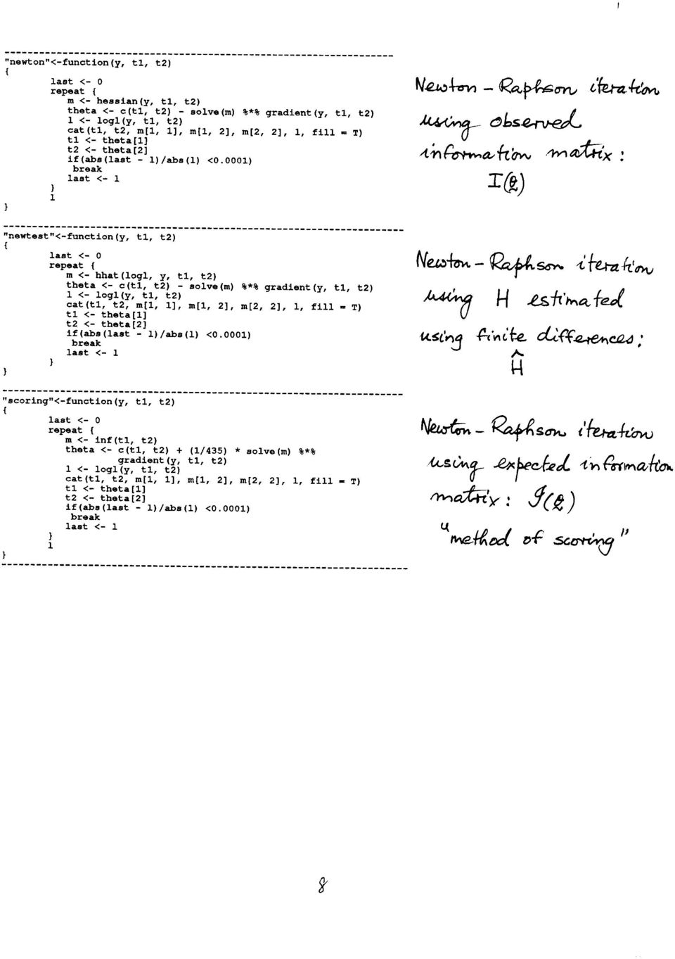
2 respectively. Asymptotically, these four forms of the information matrix can be shown to be equivalent. From a computational standpoint, the above quantities are related to those computed to solve an optimization problem as follows: l(θ corresponds to the objective function to be minimized, u(θ represents the gradient vector, the vector of first-order partial derivatives, usually denoted by g, and I(θ, corresponds to the negative of the Hessian matrix H(θ, the matrix of second-order derivatives of the objective function, respectively. In the MLE problem, the Hessian matrix is used to determine whether the minimum of the objective function l(θ is achieved by the solution ˆθ to the equations u(θ 0, i.e., whether ˆθ is a stationery point of l(θ. If this is the case, then ˆθ is the maximum likelihood estimate of θ and the asymptotic covariance matrix of ˆθ is given by the inverse of the negative of the Hessian matrix evaluated at ˆθ, which is the same as I(ˆθ, the observed information matrix evaluated at ˆθ. Sometimes it is easier to use the observed information matrix I(ˆθ for estimating the asymptotic covariance matrix of ˆθ, since if I(ˆθ were to be used then the expectation of I(ˆθ needs to be evaluated analytically. However, if computing the derivatives of l(θ in closed form is difficult or if the optimization procedure does not produce an estimate of the Hessian as a byproduct, estimates of the derivatives obtained using finite difference methods may be substituted for I(ˆθ. Newton-Raphson method is widely used for function optimization. Recall that the iterative formula for finding a maximum or a minimum of f(x was given by x (i+1 x (i H 1 (i g (i, where H (i is the Hessian f (x (i and g (i is the gradient vector f (x (i of f(x at the i th iteration. The Newton-Raphson method requires that the starting values be sufficiently close to the solution to ensure convergence. Under this condition the Newton-Raphson iteration converges quadratically to at least a local optimum. When Newton-Raphson method is applied to the problem of maximizing the likelihood function the i th iteration is given by ˆθ (i+1 ˆθ (i H(ˆθ (i 1 u(ˆθ (i. We shall continue to use the Hessian matrix notation here instead of replacing it with I(θ. Observe that the Hessian needs to be computed and inverted at every step of the iteration. In difficult cases when the Hessian cannot be evaluated in closed form, it may be substituted by a discrete estimate obtained using finite difference methods as mentioned above. In either case, computation of the Hessian may end up being a substantially large computational burden. When the expected information matrix I(θ can be derived analytically without too much difficulty, i.e., the expectation can be expressed as closed form expressions for the elements of I(θ, and hence I(θ 1, it may be substituted in the above iteration to obtain the modified iteration ˆθ (i+1 ˆθ (i + I(ˆθ (i 1 u(ˆθ (i. This saves on the computation of H(ˆθ because functions of the data y are not involved in the compuitation of I(ˆθ (i as they are with the computation of H(ˆθ. This provides a sufficiently 2

3 accurate Hessian to correctly orient the direction to the maximum. This procedure is called the method of scoring, and can be as effective as Newton-Raphson for obtaining the maximum likelihood estimates iteratively. Example 1: Let y 1,..., y n be a random sample from N(µ, σ 2, < µ <, 0 < σ 2 <. Then giving L(µ, σ 2 y n 1 (2π 1/2 σ exp [ (y i µ 2 /2σ 2] 1 (2π n/2 σ exp [ (y n i µ 2 /2σ 2] l(µ, σ 2 logl(µ, σ 2 y n logσ (y i µ 2 /2σ 2 + constant. The first partial derivatives are: l µ 2Σ(y i µ 2σ 2 Setting them to zero, l σ 2 Σ(y i µ 2 2σ 4 n 2σ 2 yi n µ 0 and (yi µ 2 /2σ 4 n/2σ 2 0, give the m.l.e. s ˆµ ȳ, and ˆσ 2 (y i ȳ 2 /n, respectively. The observed information matrix I(θ is: I(θ { 2 l θ j θ k Σ( 1 σ 2 } Σ(y i µ σ 4 Σ(y i µ Σ(y i µ 2 + n σ 4 σ 6 2σ 4 n σ 2 Σ(y i µ σ 4 Σ(y i µ Σ(y i µ 2 n σ 4 σ 6 2σ 4 and the expected information matrix I(θ is: I(θ [ n ] [ 0 n σ 0 2 nσ 0 2 n σ 2 n 0 σ 6 2σ 4 2σ 4 I(θ 1 [ σ 2 ] 0 n 2σ 0 4 n ] 3

4 Example 2: In this example, Fisher scoring is used to obtain the m.l.e. of θ using a sample of size n from the Cauchy distribution with density: f(x 1 π (x θ 2, < x <. The likelihood function is and the log-likelihood is ( 1 n n L(θ π (x i θ 2 logl(θ log (1 + (x i θ 2 + constant giving Information I(θ is log L θ n 2(x i θ 1 + (x i θ 2 u(θ. and therefore I(θ 2 log L θ 2 n/2 θ i+1 θ i + 2u(θ i n is the iteration formula required for the scoring method. Example 3: The following example is given by Rao (1973. The problem is to estimate the gene frequencies of blood antigens A and B from observed frequencies of four blood groups in a sample. Denote the gene frequencies of A and B by θ 1 and θ 2 respectively, and the expected probabilities of the four blood group O, A, B and AB by π 1, π 2, π 3, and π 4. These probabilities are functions of θ 1 and θ 2 and are given as follows: π 1 (θ 1, θ 2 2θ 1 θ 2 π 2 (θ 1, θ 2 θ 1 (2 θ 1 2θ 2 π 3 (θ 1, θ 2 θ 2 (2 θ 2 2θ 1 π 4 (θ 1, θ 2 (1 θ 1 θ 2 2 The joint distribution of the observed frequencies y 1, y 2, y 3, y 4 is a multinomial with n y 1 + y 2 + y 3 + y 4. f(y 1, y 2, y 3, y 4 n! y 1!y 2!y 3!y 4! πy 1 1 π y 2 2 π y 3 3 π y

5 It follows that the log-likelihood can be written as log L(θ y 1 log π 1 + y 2 log π 2 + y 3 log π 3 + y 4 log π 4 + constant. The likelihood estimates are solutions to log L(θ θ i.e., u(θ ( T ( π log L(θ 0 θ π ( 4 πj (y j /π j 0, θ j1 where π (π 1, π 2, π 3, π 4 T, θ (θ 1, θ 2 T, and ( π 1 2 θ θ2 2 θ 1, π ( 2 2 (1 θ θ1 θ 2 2θ 1, π ( 3 θ 2θ 2 2(1 θ 1 θ 2 The Hessian of the log-likelihood function is the 2 2 matrix:, π ( 4 2(1 θ θ1 θ 2 2(1 θ 1 θ 2. H(θ θ ( log L(θ θ [ 4 (y j /π j ( ( πj πj + j1 θ θ θ ( 4 πj (y j /π j H j (θ (y j /πj 2 j1 θ ( 4 y j (1/π j H j (θ (1/πj 2 πj j1 θ ] θ (y j/π j ( T πj θ ( πj θ T where H j (θ ( 2 π j θ h θ k is the 2 2 Hessian of πj, j 1, 2, 3, 4. These are easily computed by differentiation of the gradient vectors above: H 1 ( , H 2 ( The information matrix is then given by: ( 0 2, H 3 2 2, H 4 ( I(θ E { 2 log(θ θ j θ k } ( 4 n π j (1/π j H j (θ (1/πj 2 πj j1 θ ( ( 4 T πj πj n (1/π j j1 θ θ ( T πj θ Thus elements of I(θ can be expressed as closed form functions of θ. In his discussion, Rao gives the data as y 1 17, y 2 182, y 3 60, y and n y 1 + y 2 + y 3 + y

6 The first step in using iterative methods for computing m.l.e. s is to obtain starting values for θ 1 and θ 2. Rao suggests some methods for providing good estimates. A simple choice is to set π 1 y 1 /n, π 2 y 2 /n and solve for θ 1 and θ 2. This gives θ (0 (0.263, Three methods are used below for computing m.l.e. s; method of scoring, Newton-Raphson with analytical derivatives and, Newton-Raphson with numerical derivatives, and results of several iterations are tabulated: Table 1: Convergence of iterative methods for computing maximum likelihood estimates. (a Method of Scoring Iteration No. θ 1 θ 2 I 11 I 12 I 22 log L(θ (b Newton s Method with Hessian computed directly using analytical derivatives Iteration No. θ 1 θ 2 H 11 H 12 H 22 log L(θ (c Newton s Method with Hessian computed numerically using finite differences Iteration No. θ 1 θ 2 Ĥ 11 Ĥ 12 Ĥ 22 log L(θ

7

8

9

10

11 Using nlm( to maximize loglikelihood in the Rao example % Set-up function to return negative loglikelihood loglfunction(t { p1 2 * t[1] * t[2] p2 t[1] * (2 - t[1] - 2 * t[2] p3 t[2] * (2 - t[2] - 2 * t[1] p4 (1 - t[1] - t[2]^2 return( - (17 * log(p * log(p * log(p * log(p4 } % Use nlm( to minimize negative loglikelihood > nlm(logl,c(.263,.074,hessiant,print.level2 iteration 0 [1] 0 0 [1] [1] [1] iteration 1 [1] [1] [1] [1] iteration 2 [1] [1] [1] [1]

12 iteration 3 [1] [1] [1] [1] iteration 4 [1] e e-05 [1] [1] [1] iteration 5 [1] e e-05 [1] [1] [1] iteration 6 [1] e e-06 [1] [1] [1] iteration 7 [1] e e-06 [1] [1] [1]

13 iteration 8 [1] [1] [1] e e-05 Relative gradient close to zero. Current iterate is probably solution. $minimum [1] $estimate [1] $gradient [1] e e-05 $hessian [,1] [,2] [1,] [2,] $code [1] 1 $iterations [1] 8 Warning messages: 1: NaNs produced in: log(x 2: NaNs produced in: log(x 3: NA/Inf replaced by maximum positive value 4: NaNs produced in: log(x 5: NaNs produced in: log(x 6: NA/Inf replaced by maximum positive value 7: NaNs produced in: log(x 8: NaNs produced in: log(x 9: NA/Inf replaced by maximum positive value 13

14 Generalized Linear Models: Logistic Regression In generalized linear models (GLM s, a random variable y i from a distribution that is a member of the scaled exponential family is modelled as a function of a dependent variable x i. This family is of the form f(y θ exp {[yθ b(θ]/a(φ + c(y, θ} where θ is called the natural (or canonical parameter and φ is the scale parameter. Two useful properties of this family are E(Y b (θ V ar(y b (θ(φ The linear part of the GLM comes from the fact that some function g( of the mean E(Y i x i is modelled as a linear function x T β i.e. g(e(y i x i x T β This function g( is called the link function and is dependent on the distribution of y i. The logistic regression model is an example of a GLM. Suppose that (y i x i i 1,..., n represent a random sample from the Binomial distribution with parameters n i and p i i.e., Bin(n i, p i. Then ( n f(y p p y (1 p n y y (1 p n p ( 1 p y ( n y Thus the natural parameter is θ log ( p log ( n y. p exp {y log ( + n log (1 p + log 1 p 1 p ( n } y, a(φ 1, b(θ n log (1 p, and c(y, φ Logistic Regression Model: Lety i x i Binomial (n i, p i Then the model is: log It can be derived from this model that p i p i 1 p i β 0 + β 1 x i, i 1,..., n eβ 0 +β 1 x i 1 and thus 1 p 1+e β 0 +β 1 x i i 1+e β 0 +β 1 x i The likelihood of p is: L(p y ( k ni y i p y i i (1 p i n i y i and the log likelihood is: l(p [ ( k ni log y i + y i log p i + (n i y i log(1 p i ] 14

15 where p i are as defined above. There are two possible approaches for deriving the gradient and the Hessian. First, one can substitute p i in l above and obtain the log likelihood as a function of β: [ ( ] k ni l(β log n i log(1 + exp (β 0 + β 1 x i + y i (β 0 + β 1 x i y i and then calculate the gradient and the Hessian of l(β with respect to β directly i.e. compute l β 0, l β 1, 2 l β 0 β 1,... etc., directly or use the chain rule l β j l p i p i β j, j 0, 1 to calculate the partials from the original model as follows: log p i 1 p i β 0 + β 1 x i log p i log(1 p i β 0 + β 1 x i ( pi pi 1 p i β 0 giving p i β 0 p i (1 p i ( 1 pi p i pi x i β 1 So, after substitution, it follows that: l β 0 k k giving p i β 1 p i (1 p i { yi (n } i y i pi p i 1 p i β 0 { yi (n } i y i p i (1 p i p i 1 p i l β 1 k (y i n i p i k { yi (n } i y i p i (1 p i x i p i 1 p i k x i (y i n i p i 2 l β 2 0 k p i k n i n i p i (1 p i β 0 2 l β 0 β 1 k n i p i (1 p i x i 2 l β 2 1 k n i x i p i (1 p i x i k n i p i (1 p i x 2 i In the following implementations of Newton-Raphson, a negative sign is inserted in front of the log likelihood, the gradient, and the hessian, as these routines are constructed for minimizing nonlinear functions. 15

16 Logistic Regression using an R function I wrote for implementing Newton-Raphson using analytical derivatives Starting Values: Current Value of Log Likelihood: Current Estimates at Iteration 1 : Beta Gradient Hessian Current Value of Log Likelihood: Current Estimates at Iteration 2 : Beta Gradient Hessian Current Value of Log Likelihood: Current Estimates at Iteration 3 : Beta Gradient e e-05 Hessian Current Value of Log Likelihood: Convergence Criterion of 1e-05 met for norm of estimates. Final Estimates Are: Final Value of Log Likelihood: Value of Gradient at Convergence: e e-05 Value of Hessian at Convergence: [,1] [,2] [1,] [2,]

17 Logistic Regression: Using the R function nlm( without specifying analytical derivatives. In this case nlm( will use numerical derivatives. First, define (the negative of the log likelihood: funfunction(b,xx,yy,nn { b0 b[1] b1 b[2] cb0+b1*xx dexp(c pd/(1+d ed/(1+d^2 f -sum(log(choose(nn,yy-nn*log(1+d+yy*c return(f } Data: > x [1] > y [1] > n [1] > nlm(fun,c(-3.9,.64,hessiant,print.level2,xxx,yyy,nnn iteration 0 [1] 0 0 [1] [1] [1] iteration 1 [1] [1] [1] [1]

18 iteration 2 [1] [1] [1] [1] iteration 3 [1] [1] [1] [1] iteration 4 [1] [1] [1] [1] iteration 5 [1] [1] [1] [1] iteration 6 [1] [1] [1] [1]

19 iteration 7 [1] [1] [1] [1] iteration 8 [1] [1] [1] [1] iteration 9 [1] [1] [1] [1] iteration 10 [1] [1] [1] [1] iteration 11 [1] [1] [1] [1]

20 iteration 12 [1] e e-05 [1] [1] [1] e e-05 iteration 13 [1] [1] [1] e e-06 Relative gradient close to zero. Current iterate is probably solution. $minimum [1] $estimate [1] $gradient [1] e e-06 $hessian [,1] [,2] [1,] [2,] $code [1] 1 $iterations [1] 13 Note: The convergence criterion was determined using the default parameter values for ndigit, gradtol, stepmax, gradtol, and iterlim. 20

21 Logistic Regression Example: Solution using user written R function for computing the Loglikelihood with gradient and Hessian attributes. derfs4function(b,xx,yy,nn { b0 b[1] b1 b[2] cb0+b1*xx dexp(c pd/(1+d ed/(1+d^2 f -sum(log(choose(nn,yy-nn*log(1+d+yy*c attr(f,"gradient"c(-sum(yy-nn*p,-sum(xx*(yy-nn*p attr(f,"hessian"matrix(c(sum(nn*e,sum(nn*xx*e,sum(nn*xx*e, sum(nn*xx^2*e,2,2 return(f } > x [1] > y [1] > n [1] > nlm(derfs4,c(-3.9,.64, hessiant, iterlim500, xxx, yyy, nnn $minimum [1] $estimate [1] $gradient [1] e e-05 $hessian [,1] [,2] [1,] [2,] $code [1] 2 $iterations [1]

22 Logistic Example: Solution using nlm( and symbolic derivatives obtained from deriv3( The following statement returns a function loglik(b, x, y, nn with gradient and hessian attributes > loglikderiv3(y~(nn*log(1+exp(b0+b1*x yy*(b0+b1*x,c("b0","b1", + function(b,x,y,nn{} Save the function in you working directory as a text file by the name loglik.r > dump("loglik","loglik.r" Now edit this file by inserting the hi-lited stuff: loglik <-function (b, x, y, nn { b0 b[1] b1 b[2].expr2 <- b0 + b1 * x.expr3 <- exp(.expr2.expr4 <- 1 +.expr3.expr9 <-.expr3/.expr4.expr13 <-.expr4^2.expr17 <-.expr3 * x.expr18 <-.expr17/.expr4.value <- sum(nn * log(.expr4 - y *.expr2.grad <- array(0, c(length(.value, 2, list(null, c("b0", "b1".hessian <- array(0, c(length(.value, 2, 2, list(null, c("b0", "b1", c("b0", "b1".grad[, "b0"] <- sum(nn *.expr9 - y.hessian[, "b0", "b0"] <- sum(nn * (.expr9 -.expr3 *.expr3/.expr13.hessian[, "b0", "b1"] <-.hessian[, "b1", "b0"] <- sum(nn * (.expr18 -.expr3 *.expr17/.expr13.grad[, "b1"] <- sum(nn *.expr18 - y * x.hessian[, "b1", "b1"] <- sum(nn * (.expr17 * x/.expr4 -.expr17 *.expr17/.expr13 attr(.value, "gradient" <-.grad attr(.value, "hessian" <-.hessian.value } 22

23 > xx [1] > yy [1] > nn [1] > The number of iterations recquired for convergence by nlm( is determined by the quantities specified for the parameters ndigit, gradtol, stepmax, steptol, and iterlim. Here, using the defaults it required 338 iterations to converge. > nlm(loglik,c(-3.9,.64, hessiant, iterlim500,xxx, yyy, nnnn $minimum [1] $estimate [1] $gradient [1] e e-05 $hessian [,1] [,2] [1,] [2,] $code [1] 2 $iterations [1]

24 Concentrated or Profile Likelihood Function The most commonly used simplification in maximum likelihood estimation is the use of a concentrated or profile likelihood function. The parameter vector is first partitioned into two subsets α and β (say, of dimensions p and q, respectively and then the log-likelihood function is rewritten with two arguments, l(θ l(α, β. Now suppose that, for a given value of β, the MLEs for the subset α could be found as a function of β; that is, ˆα ˆα(β. Then the profile likelihood function is a function only of β, l c (β l [ ˆα(β, β]. (1 Clearly, maximizing l c for β will maximize l(α, β with respect to both α and β. The main advantage is a reduction in the dimension of the optimization problem. The greatest simplifications occur when ˆα does not functionally depend on β. For the first example, consider the basic problem Y i IIDN(µ, σ 2 for i 1,..., n. Then ˆµ Ȳ and is independent of σ 2 and we have l c (σ (n/2 log σ 2 (Y i Ȳ 2 /(2σ 2 This needs to be maximized only with respect to σ 2, which simplifies the problem substantially, because it is a univariate problem. For another example, consider a modification of the simple linear regression model y i α 1 + α 2 x β i + e i, e i IID N(0, α 3. (2 Given β b, the usual regression estimates can be found for α 1, α 2, α 3, but these will all be explicit functions of b. In fact, l c (β will depend only on an error sum of squares, since ˆα 3 SSE/n. Hence the concentrated likelihood function becomes simply l c (β constant n ( SSE(β 2 log. (3 n The gain is that the dimension of an unconstrained (or even constrained search has been reduced from three (or four dimensions to only one, and 1-dimensional searches are markedly simpler than those in any higher dimension. Examples: Bates and Watts (1988, p.41 gave an example of a rather simple nonlinear regression problem with two parameters: y i θ 1 (1 exp { θ 2 x i } + e i. Given θ 2, the problem becomes regression through the origin. The estimator of θ 1 is simply n / ˆθ n 1 z i y i zi 2 where z i 1 exp { θ 2 x i }, and the concentrated likelihood function is as in (3 with SSE(θ 2 Finding mle s of a two-parameter gamma distribution f(y α, β n [ yi ˆθ 1 (θ 2 ] 2. 1 β α Γ(α yα 1 exp ( y/β, for α, β, and, y > 0 24

25 provides another example. For a sample size n, the log likelihood is n l(α, β nα log(β n log Γ(α (1 α log(y i For a fixed value of α, the mle of β is easily found to be ˆβ(α n y i /nα. Thus the profile likelihood is n n l c (α nα(log( y i log(nα n log Γ(α (1 α log(y i nα A contour plot of the 2-dimensional log likelihood surface corresponding to the cardiac data, and the 1-dimensional plot of the profile likelihood are produced below. n y i β. Contour Plot of Gamma Log Likelihood Beta Alpha Plot of Profile Likelihood for Cardiac Data Profile Likelihood Alpha 25