Trading Basket Construction. Mean Reversion Trading. Haksun Li

Transcription

1 Trading Basket Construction Mean Reversion Trading Haksun Li

2 Speaker Profile Dr. Haksun Li CEO, Numerical Method Inc. (Ex-)Adjunct Professors, Industry Fellow, Advisor, Consultant with the National University of Singapore, Nanyang Technological University, Fudan University, the Hong Kong University of Science and Technology. Quantitative Trader/Analyst, BNPP, UBS PhD, Computer Sci, University of Michigan Ann Arbor M.S., Financial Mathematics, University of Chicago B.S., Mathematics, University of Chicago 2

3 References Pairs Trading: A Cointegration Approach. Arlen David Schmidt. University of Sydney. Finance Honours Thesis. November Likelihood-Based Inference in Cointegrated Vector Autoregressive Models. Soren Johansen. Oxford University Press, USA. February 1, Pairs Trading. Elliot, van der Hoek, and Malcolm Identifying Small Mean Reverting Portfolios. A. d'aspremont High-frequency Trading. Stanford University. Jonathan Chiu, Daniel Wijaya Lukman, Kourosh Modarresi, Avinayan Senthi Velayutham

4 4 Paris Trading

5 Pairs Trading Intuition: The thousands of market instruments are not independent. For two closely related assets, they tend to move together (common trend). We want to buy the cheap one and sell the expensive one. Exploit short term deviation from long term equilibrium. Definition: trade one asset (or basket) against another asset (or basket) Long one and short the other Try to make money from spread. 5

6 FOMC announcements Rate cut! Bonds react. FX react. Stocks react. All act! 6

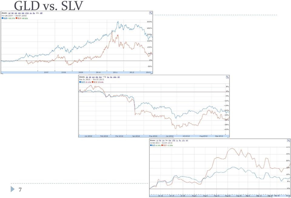
7 GLD vs. SLV 7

8 Hows How to construct a pair? How to trade a pair? 8

9 9 Sample Pairs Trading Strategy

10 Spread Z = X βy β hedge ratio Cointegration coefficient How do you trade spread? How much X to buy/sell? How much Y to buy/sell? 10

11 Log-Spread Z = log X β log Y How do you trade log-spread? How much X to buy/sell? How much Y to buy/sell? 11

12 Dollar Neutral Hedge Suppose ES (S&P500 E-mini future) is at 1220 and each point worth $50, its dollar value is about $61,000. Suppose NQ (Nasdaq 100 E-mini future) is at 1634 and each point worth $20, its dollar value is $32,680. β = = Z = EE 1.87 NN Buy Z = Buy 10 ES contracts and Sell 19 NQ contracts. Sell Z = Sell 10 ES contracts and Buy 19 NQ contracts. 12

13 Market Neutral Hedge Suppose ES has a market beta of 1.25, NQ We use β = =

14 Dynamic Hedge β changes with time, covariance, market conditions, etc. Periodic recalibration. 14

15 Distance Method The distance between two time series: d = x i y j 2 x i, y j are the normalized prices. We choose a pair of stocks among a collection with the smallest distance, d. 15

16 Distance Trading Strategy Sell Z if Z is too expensive. Buy Z if Z is too cheap. How do we do the evaluation? 16

17 Z Transform We normalize Z. The normalized value is called z-score. z = x x σ x Other forms: z = x M x S σ x M, S are proprietary functions for forecasting. 17

18 A Very Simple Distance Pairs Trading Sell Z when z > 2 (standard deviations). Sell 10 ES contracts and Buy 19 NQ contracts. Buy Z when z < -2 (standard deviations). Buy 10 ES contracts and Sell 19 NQ contracts. 18

19 Pros of the Distance Model Model free. No mis-specification. No mis-estimation. Distance measure intuitively captures the Law of One Price (LOP) idea. 19

20 Cons of the Distance Model There is no reason why the model will work (or not). There is no assumption to check against the current market conditions. The model is difficult to analyze mathematically. Cannot predict the convergence time (expected holding time). The model ignores the dynamic nature of the spread process, essentially treating the spread as i.i.d. Using more strict criterions may work for equities. In FX trading, we don t have the luxury of throwing away many pairs. 20

21 Risks in Pairs Trading Long term equilibrium does not hold. E.g., the company that you long goes bankrupt but the other leg does not move (one company wins over the other). Systematic market risk. Firm specific risk. Liquidity. 21

22 22 Cointegration

23 Stationarity These ad-hoc βcalibration does not guarantee the single most important statistical property in trading: stationarity. Strong stationarity: the joint probability distribution of x t does not change over time. Weak stationarity: the first and second moments do not change over time. Covariance stationarity 23

24 Mean Reversion A stationary stochastic process is mean-reverting. Long when the spread/portfolio/basket falls sufficiently below a long term equilibrium. Short when the spread/portfolio/basket rises sufficiently above a long term equilibrium. 24

25 Test for Stationarity An augmented Dickey Fuller test (ADF) is a test for a unit root in a time series sample. It is an augmented version of the Dickey Fuller test for a larger and more complicated set of time series models. Intuition: if the series y t is stationary, then it has a tendency to return to a constant mean. Therefore large values will tend to be followed by smaller values, and small values by larger values. Accordingly, the level of the series will be a significant predictor of next period's change, and will have a negative coefficient. If, on the other hand, the series is integrated, then positive changes and negative changes will occur with probabilities that do not depend on the current level of the series. In a random walk, where you are now does not affect which way you will go next. 25

26 ADF Math p 1 i=1 Δy t i Δy t = α + ββ + γy t ε t Null hypothesis H 0 : γ = 0. (y t non-stationary) α = 0, β = 0 models a random walk. β = 0 models a random walk with drift. Test statistics = γ σ γ, the more negative, the more reason to reject H 0 (hence y t stationary). SuanShu: AugmentedDickeyFuller.java 26

27 Cointegration Cointegration: select a linear combination of assets to construct an (approximately) stationary portfolio. 27

28 Objective Given two I(1) price series, we want to find a linear combination such that: z t = x t βy t = μ + ε t ε t is I(0), a stationary residue. μ is the long term equilibrium. Long when z t < μ Δ. Sell when z t > μ + Δ. 28

29 Stocks from the Same Industry Reduce market risk, esp., in bear market. Stocks from the same industry are likely to be subject to the same systematic risk. Give some theoretical unpinning to the pairs trading. Stocks from the same industry are likely to be driven by the same fundamental factors (common trends). 29

30 Cointegration Definition X t ~CI d, b if All components of X t are integrated of same order d. There exists a β t such that the linear combination, β t X t = β 1 X 1t + β 2 X 2t + + β n X nt, is integrated of order d b, b > 0. β is the cointegrating vector, not unique. 30

31 Illustration for Trading Suppose we have two assets, both reasonably I(1), we want to find β such that Z = X + βy is I(0), i.e., stationary. In this case, we have d = 1, b = 1. 31

32 A Simple VAR Example y t = a 11 y t 1 + a 12 z t 1 + ε yy z t = a 21 y t 1 + a 22 z t 1 + ε zt Theorem 4.2, Johansen, places certain restrictions on the coefficients for the VAR to be cointegrated. The roots of the characteristics equation lie on or outside the unit disc. 32

33 Coefficient Restrictions a 11 = 1 a 22 a 12 a 21 1 a 22 a 22 > 1 a 12 a 21 + a 22 < 1 33

34 VECM (1) Taking differences y t y t 1 = a 11 1 y t 1 + a 12 z t 1 + ε yy z t z t 1 = a 21 y t 1 + a 22 1 z t 1 + ε zt Δy t Δz t = a 11 1 a 12 a 21 a 22 1 y t 1 z t 1 + ε yy ε zt Substitution of a 11 Δy t Δz t = a 12 a 21 1 a 22 a 12 a 21 a 22 1 y t 1 z t 1 + ε yy ε zt 34

35 VECM (2) Δy t = α y y t 1 βz t 1 Δz t = α z y t 1 βz t 1 α y = a 12a 21 1 a 22 + ε yy + ε zt α z = a 21 β = 1 a 22, the cointegrating coefficient a 21 y t 1 βz t 1 is the long run equilibrium, I(0). α y, α z are the speed of adjustment parameters. 35

36 Interpretation Suppose the long run equilibrium is 0, Δy t, Δz t responds only to shocks. Suppose α y < 0, α z > 0, y t decreases in response to a +ve deviation. z t increases in response to a +ve deviation. 36

37 Granger Representation Theorem If X t is cointegrated, an VECM form exists. The increments can be expressed as a functions of the dis-equilibrium, and the lagged increments. ΔX t = αβ X t 1 + c t ΔX t 1 + ε t In our simple example, we have Δy t Δz t = α y α z 1 β y t 1 z t 1 + ε yy ε zt 37

38 Granger Causality z t does not Granger Cause y t if lagged values of Δz t i do not enter the Δy t equation. y t does not Granger Cause z t if lagged values of Δy t i do not enter the Δz t equation. 38

39 Engle-Granger Two Step Approach Estimate either y t = β 10 + β 11 z t + e 1t z t = β 20 + β 21 y t + e 2t As the sample size increase indefinitely, asymptotically a test for a unit root in e 1t and e 2t are equivalent, but not for small sample sizes. Test for unit root using ADF on either e 1t and e 2t. If y t and z t are cointegrated, β super converges. 39

40 Engle-Granger Pros and Cons Pros: simple Cons: This approach is subject to twice the estimation errors. Any errors introduced in the first step carry over to the second step. Work only for two I(1) time series. 40

41 Testing for Cointegration Note that in the VECM, the rows in the coefficient, Π, are NOT linearly independent. Δy t Δz t = a 12 a 21 1 a 22 a 12 a 21 a 22 1 y t 1 z t 1 + ε yy ε zt a 12a 21 1 a 22 a 12 1 a 22 a 12 = a 21 a 22 1 The rank of Π determine whether the two assets y t and z t are cointegrated. 41

42 VAR & VECM In general, we can write convert a VAR to an VECM. VAR (from numerical estimation by, e.g., OLS): X t = p i=1 A i X t i + ε t Transitory form of VECM (reduced form) ΔX t = ΠX t 1 + p 1 i=1 Long run form of VECM ΔX t = p 1 i=1 Υ i ΔX t i Γ i ΔX t i + ε t + ΠX t p + ε t 42

43 The Π Matrix Rank(Π) = n, full rank The system is already stationary; a standard VAR model in levels. Rank(Π) = 0 There exists NO cointegrating relations among the time series. 0 < Rank(Π) < n Π = αβ β is the cointegrating vector α is the speed of adjustment. 43

44 Rank Determination Determining the rank of Π is amount to determining the number of non-zero eigenvalues of Π. Π is usually obtained from (numerical VAR) estimation. Eigenvalues are computed using a numerical procedure. 44

45 Trace Statistics Suppose the eigenvalues of Π are:λ 1 > λ 2 > > λ n. For the 0 eigenvalues, ln 1 λ i = 0. For the (big) non-zero eigenvalues, ln 1 λ i is (very negative). The likelihood ratio test statistics p Q H r H n = T i=r+1 log 1 λ i H0: rank r; there are at most r cointegrating β. 45

46 Test Procedure int r = 0;//rank for (; r <= n; ++r) { // loop until the null is accepted } compute Q = Q H r H n ; If (Q > c.v.) { // compare against a critical value } break; // fail to reject the null hypothesis; rank found r is the rank found 46

47 Decomposing Π Suppose the rank of Π = r. Π = αβ. Π is n n. α is n r. β is r n. 47

48 Estimating β β can estimated by maximizing the log-likelihood function in Chapter 6, Johansen. logl Ψ, α, β, Ω Theorem 6.1, Johansen: β is found by solving the following eigenvalue problem: λs 11 S 10 S 00 1 S 01 = 0 48

49 β Each non-zero eigenvalue λ corresponds to a cointegrating vector, which is its eigenvector. β = v 1, v 2,, v r β spans the cointegrating space. For two cointegrating asset, there are only one β (v 1 ) so it is unequivocal. When there are multiple β, we need to add economic restrictions to identify β. 49

50 Trading the Pairs Given a space of (liquid) assets, we compute the pairwise cointegrating relationships. For each pair, we validate stationarity by performing the ADF test. For the strongly mean-reverting pairs, we can design trading strategies around them. 50

51 Problems with Using Cointegration The assets may be cointegrated sometimes but not always. What do you do when it is not cointegrated but you are already in the market? Cointegration creates a dense basket it includes every asset in the time series analyzed. Incur huge transaction cost. Reduce the significance of the structural relationships. Optimal mean reverting portfolios behave like noise and vary well inside the bid-ask spreads, hence not meaningful statistical arbitrage opportunities. What about not so optimal ones? 51

52 52 Stochastic Spread

53 Ornstein Uhlenbeck Process z t = x t βy t dz t = θ μ z t dd + σσw t 53

54 Spread as a Mean-Reverting Process x k x k 1 = = b a b x k 1 a bx k 1 τ + σ τε k τ + σ τε k The long term mean = a b. The rate of mean reversion = b. 54

55 Sum of Power Series We note that = k 1 i=0 a i = ak 1 a 1 55

56 Unconditional Mean E x k = μ k = μ k 1 + a bμ k 1 τ = aτ + 1 bτ μ k 1 = aτ + 1 bτ aτ + 1 bτ μ k 2 = aτ + 1 bτ aτ + 1 bτ 2 μ k 2 k 1 = i=0 1 bτ i aτ + 1 bτ k μ 0 = aτ = aτ 1 1 bτ k 1 1 bτ 1 1 bτ k bτ + 1 bτ k μ bτ k μ 0 = a b a b 1 bτ k + 1 bτ k μ 0 56

57 Long Term Mean a b a b 1 bτ k + 1 bτ k μ 0 a b 57

58 Unconditional Variance Var x k = σ k 2 = 1 bτ 2 σ k σ 2 τ = 1 bτ 2 σ k σ 2 τ = 1 bτ 2 1 bτ 2 σ k σ 2 τ + σ 2 τ k 1 = σ 2 τ i=0 1 bτ 2i + 1 bτ 2k σ 2 0 = σ 2 τ 1 1 bτ 2k 1 1 bτ bτ 2k σ

59 Long Term Variance σ 2 τ 1 1 bτ 2k 1 1 bτ bτ 2k σ 0 2 σ2 τ 1 1 bτ 2 59

60 Observations and Hidden State Process The hidden state process is: x k = x k 1 + a bx k 1 τ + σ τε k = aτ + 1 bτ x k 1 + σ τε k = A + Bx k 1 + Cε k A 0, 0 < B < 1 The observations: y k = x k + Dω k We want to compute the expected state from observations. x k = x k k = E x k Y k 60

61 Parameter Estimation We need to estimate the parameters θ = A, B, C, D from the observable data before we can use the Kalman filter model. We need to write down the likelihood function in terms of θ, and then maximize w.r.t. θ. 61

62 Likelihood Function A likelihood function (often simply the likelihood) is a function of the parameters of a statistical model, defined as follows: the likelihood of a set of parameter values given some observed outcomes is equal to the probability of those observed outcomes given those parameter values. L θ; Y = p Y θ 62

63 Maximum Likelihood Estimate We find θ such that L θ; Y is maximized given the observation. 63

64 Example Using the Normal Distribution We want to estimate the mean of a sample of size N drawn from a Normal distribution. f y = 1 y μ 2 exp 2πσ2 2σ 2 θ = μ, σ N 1 L N θ; Y = exp y i μ 2 i=1 2πσ 2 2σ 2 64

65 Log-Likelihood log L N θ; Y = N i=1 log 1 y i μ 2 2πσ 2 2σ 2 Maximizing the log-likelihood is equivalent to maximizing the following. N i=1 y i μ 2 First order condition w.r.t.,μ μ = 1 N N i=1 y i 65

66 Nelder-Mead After we write down the likelihood function for the Kalman model in terms of θ = A, B, C, D, we can run any multivariate optimization algorithm, e.g., Nelder- Mead, to search for θ. max θ L θ; Y The disadvantage is that it may not converge well, hence not landing close to the optimal solution. 66

67 Marginal Likelihood For the set of hidden states, X t, we write L θ; Y = p Y θ = p Y, X θ X Assume we know the conditional distribution of X, we could instead maximize the following. max E θ X max E θ X L θ Y, X, or log L θ Y, X The expectation is a weighted sum of the (log-) likelihoods weighted by the probability of the hidden states. 67

68 The Q-Function Where do we get the conditional distribution of X t from? Suppose we somehow have an (initial) estimation of the parameters, θ 0. Then the model has no unknowns. We can compute the distribution of X t. Q θ θ t = E X Y,θ log L θ Y, X 68

69 EM Intuition Suppose we know θ, we know completely about the mode; we can find X. Suppose we know X, we can estimate θ, by, e.g., maximum likelihood. What do we do if we don t know both θ and X? 69

70 Expectation-Maximization Algorithm Expectation step (E-step): compute the expected value of the log-likelihood function, w.r.t., the conditional distribution of X under Yand θ. Q θ θ t = E X Y,θ log L θ Y, X Maximization step (M-step): find the parameters, θ, that maximize the Q-value. θ t+1 = argmax θ Q θ θ t 70

71 EM Algorithms for Kalman Filter Offline: Shumway and Stoffer smoother approach, 1982 Online: Elliott and Krishnamurthy filter approach,

72 First Passage Time Standardized Ornstein-Uhlenbeck process dd t = Z t dd + 2dd t First passage time T 0,c = inf t 0, Z t = 0 Z 0 = c The pdf of T 0,c has a maximum value at t = 1 2 ln c c 2 + c

73 A Sample Trading Strategy x k = x k 1 + a bx k 1 τ + σ τε k dx t = a bb t dd + σdd t X 0 = μ + c σ, X T = μ 2ρ T = 1 ρ t Buy when y k < μ c Sell when y k > μ + c σ 2ρ σ 2ρ unwind after time T unwind after time T 73

74 Kalman Filter The Kalman filter is an efficient recursive filter that estimates the state of a dynamic system from a series of incomplete and noisy measurements. 74

75 Conceptual Diagram as new measurements come in prediction at time t Update at time t+1 correct for better estimation 75

76 A Linear Discrete System x k = F k x k 1 + B k u k + ω k F k : the state transition model applied to the previous state B k : the control-input model applied to control vectors ω k ~N 0, Q k : the noise process drawn from multivariate Normal distribution 76

77 Observations and Noises z k = H k x k + v k H k : the observation model mapping the true states to observations v k ~N 0, R k : the observation noise 77

78 Discrete System Diagram 78

79 Prediction predicted a prior state estimate x k k 1 = F k x k 1 k 1 + B k u k predicted a prior estimate covariance P k k 1 = F k P k 1 k 1 F k T + Q k 79

80 Update measurement residual y k = z k H k x k k 1 residual covariance S k = H k P k k 1 H k T + R k optimal Kalman gain K k = P k k 1 H k T S k 1 updated a posteriori state estimate x k k = x k k 1 + K k y k updated a posteriori estimate covariance P k k = I K k H k P k k 1 80

81 Computing the Best State Estimate Given A, B, C, D, we define the conditional variance R k = Σ k k E x k x 2 k Y k Start with x 0 0 = y 0, R 0 = D 2. 81

82 Predicted (a Priori) State Estimation x k+1 k = E x k+1 Y k = E A + Bx k + Cε k+1 Y k = E A + Bx k Y k = A + B E x k Y k = A + Bx k k 82

83 Predicted (a Priori) Variance Σ k+1 k = E x k+1 x 2 k+1 Y k = E A + BB k + Cε k+1 x 2 k+1 Y k = E 2 A + BB k + Cε k+1 A Bx k k Yk = E BB k Bx k k + Cε k+1 2 Yk = E BB k Bx k k 2 + C 2 ε 2 k+1 Y k = B 2 Σ k k + C 2 83

84 Minimize Posteriori Variance Let the Kalman updating formula be x k+1 = x k+1 k+1 = x k+1 k + K y k+1 x k+1 k We want to solve for K such that the conditional variance is minimized. Σ k+1 k = E x k+1 x k+1 2 Y k 84

85 Solve for K E x k+1 x 2 k+1 Y k 2 = E x k+1 x k+1 k K y k+1 x k+1 k Yk 2 = E x k+1 x k+1 k K x k+1 x k+1 k + Dω k+1 Yk 2 = E 1 K x k+1 x k+1 k KKω k+1 Yk = 1 K 2 2 E x k+1 x k+1 k Yk + K 2 D 2 = 1 K 2 Σ k+1 k + K 2 D 2 85

86 First Order Condition for k d dk 1 K 2 Σ k+1 k + K 2 D 2 = d dk 1 2K + K2 Σ k+1 k + K 2 D 2 = 2 + 2K Σ k+1 k + 2KD 2 = 0 86

87 Optimal Kalman Filter K k+1 = Σ k+1 k Σ k+1 k +D 2 87

88 Updated (a Posteriori) State Estimation So, we have the optimal Kalman updating rule. x k+1 = x k+1 k+1 = x k+1 k + K y k+1 x k+1 k = x k+1 k + Σ k+1 k Σ k+1 k +D 2 y k+1 x k+1 k 88

89 Updated (a Posteriori) Variance R k+1 = Σ k+1 k = E x k+1 x k+1 2 Y k+1 = 1 K 2 Σ k+1 k + K 2 D 2 = 1 Σ k+1 k Σ k+1 k +D 2 = D 2 Σ k+1 k +D Σ k+1 k + Σ k+1 k + = D4 Σ k+1 k +D 2 Σ k+1 k 2 Σ k+1 k +D 2 2 = D4 Σ k+1 k +D 2 Σ k+1 k 2 Σ k+1 k +D 2 2 = Σ k+1 kd 2 D 2 +Σ k+1 k D 2 = Σ k+1 k D 2 Σ k+1 k +D 2 2 Σ k+1 k Σ k+1 k +D 2 Σ k+1 k Σ k+1 k +D 2 2 D 2 2 D 2 89

90 A Trading Algorithm From y 0, y 1,, y N, we estimate θ N. Decide whether to make a trade at t = N, unwind at t = N + 1, or some time later, e.g., t = N + T. As y N+1 arrives, estimate θ N + 1. Repeat. 90

91 Results (1) 91

92 Results (2) 92

93 Results (3) 93