Convective Weather Maps

Transcription

1 Guide to using Convective Weather Maps Oscar van der Velde last modified: August 27th, 2007 Reproduction of this document or parts of it is allowed with permission. This document may be updated at any time. Picture taken May 13th 2007, 1706 UTC, in southwesterly direction from Toulouse, France

2 Introduction I have finally written some explanation for you about the parameters plotted in the maps and how to use them. The maps are presented on and the latter is the server hosting the maps. Many parameters are based on concepts of "parcel theory" which describes what happens to a parcel of air when brought to a different pressure, relative to their new surroundings. My purpose is not to explain all details of physical meteorology (you will find it in any meteorology textbook and also in the very good MetEd modules on the web), but how to apply the parameters plotted in the Convective Weather Maps to forecasting. I started playing around with GrADS in February 2002 with data from the AVN model from the National Center for Environmental Prediction (NCEP) which had a grid spacing of 1x1 degree. Now the maps are run from the GFS model at 0.5 degree grid. While I have always been interested in forecasting thunderstorms, almost no model output was available for Europe with useful parameters for this purpose, indicating different measures of instability, vertical wind shear, or low-level convergence. It is very important to have enough parameters available to construct a conceptual image of the timing and type of thunderstorms that are thought to occur. This is why the Storm Prediction Center in the United States has a wide variety of parameters available for this purpose (see their Meso-analysis section). Many parameters were tested on soundings (e.g. publications of Rasmussen, Brooks in Weather and Forecasting) and are proven skillful in forecasting severe thunderstorms and tornadoes, while being based on parcel theory and results from cloud-resolving modelling studies of the interaction of vertical shear with updrafts and downdrafts in thunderstorms (by researchers Wilhelmson, Weisman, Klemp and Rotunno). This knowledge is now increasingly common among those who have a strong interest in chasing or forecasting thunderstorms in particular and want to have a reasonable skill doing so. In my experience however, most national weather forecasting offices at this side of the ocean are lagging behind, while more and more statistical approaches to forecasting are taken. Statistics are fast to implement in products, but at the cost of conceptually knowing what is going on in the physical world. For example, the concept of convective modes (single cell, multicell, supercell, mesoscale convective system) is strongly tied to vertical wind shear and this can make an enormous difference in the character of thunderstorms. If a forecasting office does not pay attention to these concepts and fails to recognize important radar characteristics of ongoing storms,

3 severe weather may result without warning. I hope this document will inspire everyone to take a deeper look at the physics of severe storms, their forecasting, how to recognize them on radar, and what to do with this information for your purpose (the latter two are beyond the scope of this document). The three basic ingredients for severe deep convection are instability, lift, and vertical wind shear. In many situations, without a good source of lift (e.g. a front, trough, sea breeze convergence, dryline, forced flow over mountains) a parcel which has conditional instability will have trouble to rise out of the boundary layer and form a persisting convective storm. Without vertical shear (change of direction and speed of the horizontal wind with height) a storm will have trouble to live longer than about 45 minutes and die, instead of organizing itself into a cluster or MCS, or develop a rotating updraft, with all consequences for severe weather potential. Note: references will be added later. For a quick and entertaining crash-course in operational severe storm meteorology, I highly recommend MetEd:

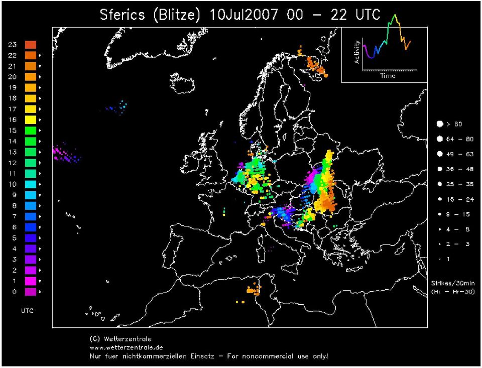
4 The Maps The examples below are from 10 July 2007, for 15Z. This day featured a cold front over eastern Europe along which severe thunderstorms developed, with a tornado at 1645 UTC in southwestern Romania, large hail over central Romania in the evening. More events likely happened along the front, but have not reached the ESWD. Supercells were visible also on Serbian radar. A typical spout situation was present over Netherlands into Germany with several complete spouts and funnels having been reported during late morning and afternoon, and a few cases of up to 2 cm hail over Germany later towards/in evening. At the time of the satellite image, the storms over western Ukraine from the early afternoon have produced a large cirrus shield already. The purpose here is only to show examples of the parameter fields, not to discuss the case in detail (refer to the forecast archive of the European Storm Forecast Experiment, A different case may be selected in a later version of the document.

5

6 1. MLCAPE (and MSL Pressure, 500 hpa Geopotential Heights) This map offers a usual view of common heights for a quick overview of pressure systems, with the addition of mixed-layer CAPE (Convectively Available Potential Energy). CAPE is the potential energy a parcel has when it is lifted to its level of free convection and becomes warmer than its surroundings, experiencing upward buoyancy. The potential energy can be converted to kinetic energy reflected in upward motion. An vertical speed could in principle be calculated from this, but parcel theory is not perfect and does not account for things like precipitation drag or dynamic pressure contributions of vertical shear. However, higher CAPE typically involves stronger storms with a higher chance of large hail and other severe weather. That said, note that CAPE is usually of lesser importance than the vertical shear environment for tornadoes, while the probability of large hail increases with CAPE, given at least moderate shear (values around J/kg are sufficient). Contributors to CAPE are steep temperature lapse rates from low to mid levels and a warm and humid boundary layer. The colder the mid levels are compared to the parcel, and the higher the parcel experiences upward buoyancy (high equilibrium level), the larger CAPE in general. However, warm, dry layers at low levels may function as a cap

7 that prevent boundary layer parcels from reaching the level of free convection, and may prevent storms from developing (see LFC-LCL map). The CAPE used in these maps is calculated for a parcel with mixing ratio and potential temperature averaged from the 0-1 km layer, because it reflects the process of mixing in the boundary layer. Note that the problem of GFS overestimating low level dewpoints (and hence CAPE) in conditions of weak winds and strong insolation in the summer half year is somewhat mitigated by not including the 2-meter level in the calculation. Finally, be aware that CAPE is very sensitive to small differences in the moisture and temperature profiles, as well as the calculation and used parcel. It is therefore fairly useless to speak for example of "855 J/kg CAPE" or even "900 J/kg". If the maps indicate 1000 J/kg CAPE, be prepared to find in soundings mostly J/kg, a wide margin of at least 50%. 2. Omega: Advection of 600 hpa Geostrophic Vorticity by the hpa Thermal Wind Vectors, 600 hpa Height This map uses the Trenberth method for estimating the resulting vertical motion induced by differential vorticity advection and temperature advection, giving a

8 qualitative picture of geostrophic vertical motions. It is different from model output vertical motions (which are influenced also by convection itself). Use to get a sense of large scale lift and subsidence. Cellular convection over sea often is able to maintain itself even under subsidence, if low level lapse rates are strong enough, but comma clouds for example would need geostrophic lift (usually a vorticity maximum). It is recommended to double-check the existence of ascent/descent with other geostrophic vertical motion parameters for critical use. 3. Mid-tropospheric Potential Vorticity ( hpa) Used to highlight atmospheric processes in a different way. PV is a conserved quantity for adiabatic processes, equivalent to momentum. It can be used to trace airmasses. The tropopause is usually associated with 2 PV units, with lower PV below. Strong vertical motions can stir up the tropopause, such that high PV air enters the troposphere and is brought downwards. The presence of a strong PV anomaly in midlevels or lower indicates either strong postfrontal subsidence or a bubble of mid-level cold air with steep lapse rates and high vorticity. I won't go deeply into PV theory, but for practical

9 use: strong upward motions can be expected ahead of a PV maximum, in other words, mid-level lapse rates will steepen and mid-level vorticity generating upward motion in the direction a PV maximum moves. Especially the dark blue and beyond needs attention. The patterns seen in this map often correspond with the dark bands in satellite water vapour images (intrusions of dry air). 4. Thompson index, Convective Precipitation, 700 hpa Height The Thompson thunderstorm index is an ancient index, from the times that every calculation had to be done be hand from soundings. The index consists of K Index minus the Lifted Index. The latter is simply the difference between the temperature a parcel has at 500 hpa and its surrounding air, so a result of parcel theory. The K Index is T850 + Td850 - (T700 - Td700) -T500 and thus a sum with no meaning, including a lapse rate, a low level dewpoint and a mid level relative humidity. The fixed levels make this physically mean something different on high plains than at sea level. But it came out best in a comparison study of a number of cases with SFLOCs (lightning reports) I did almost 10 years ago. The 700 hpa moisture factor in it can be useful for the reason that it

10 serves to indirectly include a source of lift, as usually it is more humid in the mid levels around fronts. I strongly suggest using parcel theory parameters though. What to use the map for is mainly a view of standard output GFS convective precipitation... which actually is often fairly reliable although it may overreact in case the evapo-transpiration problem (weak wind, strong insolation) shows up. It may underestimate potential for storms in areas with deep dry boundary layers. 5. Equilibrium Level Temperature (most unstable parcel) A very useful map in cases of near-neutral environments of very low CAPE, read: mostly in the winter half year. Convective cells need to have updrafts reaching sufficiently into the mixed-phase temperature region (usually -10 to -30 degrees Celsius), where ice particles in the cloud co-exist with liquid water droplets, in order for the non-inductive charging process to be effective. The equilibrium level is where the parcel will be at the same temperature as the environment after its free convection. It will experience an increasingly negative buoyancy force as it ascends further and will slow down. This often corresponds with levels near the tropopause, but may also be an

11 inversion lower in the troposhere. The map indicates the temperature, not the height. Thunder may be possible with EL temperatures lower than -10 degrees, and becomes likely especially beyond -30 degrees. In winter time the corresponding heights of the cloud tops is lower and the moisture content lower as well, with weaker updrafts so the electrification process is less effective. In the summer over large areas parcels can reach very cold temperatures and other indicators may be more useful to look at. However, for the calculation the "best layer" is used (i.e. the level with the highest theta-e parcel below 600 hpa), and this map is useful in identifying elevated convection when ML parcel methods do not show potential. Attention: there is currently no map to check the LFC of an elevated parcel. 6. Lifting Condensation Level, LFC-LCL difference The height of the LCL of a 0-1 km mixed parcel is plotted as background. This LCL is similar to the Convective Condensation Level, i.e. the cloud base height that cumuliform clouds may have. It relates strongly to the relative humidity of the boundary layer, so very low heights may associate with low clouds or fog during the

12 night (and in bad cases persist during the day and block solar heating required for storms). High LCL heights can enhance downburst winds because the downdraft air will be colder relative to the surrounding air, the negative buoycancy accelerating downward speeds. High LCLs (>2000 m) may also indicate more difficulty for beginning convection to sustain itself, due to entrainment in the dry environment. Low LCL heights (under 1000 meters) are favourable for tornadoes, as was found by SPC, the reasons of which have not been fully explained, but involve downdraft-updraft buoyancy processes. The LFC (Level of Free Convection) is the level below which a 0-1 km mixed parcel when lifted is colder than its environment, and normally wants to return to where it came from. A very strong source of low-level lift may push a parcel to the LFC, so that it becomes warmer (lighter) than the surrounding air and experience an upward force. More common is that the capping warm layer is adiabatically lifted and removed, or that heating and mixing from below will yield a higher LCL and a lower LFC (the convective temperature concept). In the form of vectors, the difference between the cloud base and the Level of Free Convection is drawn. No vector means no MLCAPE present. Small vectors indicate small LFC-LCL differences, so that there is almost no extra heating or forcing required for initiation of convection. Longer vectors require more, and thick vectors may indicate too much capping inhibiting the formation of thunderstorms. Along the dryline in the USA Great Plains, the gradient may be so steep that only a few points with small LFCLCL are visible on the grid points of the model. At night, the LFC-LCL difference may increase again, but usually already developed storms will persist for some time, depending on moisture and storm-relative inflow above the boundary layer. In general, the lower the LFC-LCL difference, the easier (less forcing required) and earlier storms develop. The same goes for lower LCLs because entrainment is less of a problem. Note that because the model adjusts its environment (weakens lapse rates, lowers LCL) as result of convection, the LFC-LCL difference may become larger and may give a counter-intuitive capped impression where there is already convection. Check this by looking at the convective precipitation map.

13 km MLCAPE, Spout index 0-3 km MLCAPE (low-level CAPE) uses the 0-1 km mixed layer parcel, but represents the MLCAPE present not all the way to the EL, but only in the lowest three kilometers above the surface. This indicates whether a parcel is able to accelerate rapidly above the LFC. A low LFC and temperatures dropping rapidly with height in the 0-3 km layer make for a upward acceleration in this layer, which is important especially for tornadogenesis. The type of generally weak tornadoes (F0-F1) known as 'spouts' (landspouts, waterspouts) happen by stretching of vorticity with a vertical axis into an updraft. This process is enhanced by vertical acceleration (the same mechanism as the whirl when draining water from a bathtub). Prerequisite is a source of vertical vorticity and convergence, such as wind shift lines. In addition it seems important that low-level winds are not too strong, otherwise turbulence may disturb this process. Steep nearsurface lapse rates will also help (next map). Mid/upper level cold pools and weak troughs are notorious for outbreaks of spouts. The green experimental composite index incorporates these factors, but it is not calibrated or tested, and may not always be useful.

14 Similarly, tornadoes can be generated by tilting of low-level vorticity with a horizontal axis (strong low-level shear) into the vertical by a strong updraft and may also profit from stronger 0-3 km CAPE. 8. Temperature Lapse Rate: m AGL The temperature difference between the surface (not 2 meters) and 500 m above ground. This map contains useful information about the relative temperature of the air compared to the surface over which it flows. The dry-adiabatic lapse rate is about Kelvin decrease per kilometer, while 5-6 degrees decrease per kilometer is moistadiabatic. Lower values indicate inversions. Values higher than 11 K/km indicate superadiabatic conditions which necessarily imply turbulent mixing as surface parcels have already positive buoyancy with the minimal lift. This is favourable for vertical vortex stretching such as dust devils and spouts. One may often easily infer which process is responsible for steep or inverted lapse rates. Large bodies of water do not change temperature very quickly, so very steep lapse rates will mostly be the result of advection of relatively cold air over the surface. Similarly,

15 inverted lapse rates indicate strong warm air advection over the water surface. Land, on the other hand, responds quickly to radiative processes. Contrasts between land and adjacent water surfaces may induce mesoscale circulations like land/sea breeze. Lapse rates increase quickly during the afternoon when the sun shines, while in the evening a ground inversion forms. This makes it possible to evaluate if the model produces cloudiness that may inhibit heating of the boundary layer during the day, or reflect of long wave radiation to earth at night (>4 K/km over land), making it a useful map if also if you need to know possibilities for clear skies at night for astronomical observations or sprites. 9. Temperature Lapse Rate: m AGL This somewhat arbitrarily chosen layer for mid-level lapse rates is often used to identify an important contributor to CAPE, independently of moisture availability. In maritime polar airmasses behind cold fronts it generally indicates values over 6 K/km. More equatorward it often is capable of defining the edge of deep convection rather well, where subsidence establishes an inversion. Shallow convection may still occur in these

16 regions. Elevated and dry regions such as the Spanish Plateau and the Sahara often create a deep dry layer with steep lapse rates, that can be advected away into western Europe (e.g. Spanish Plume). On the Great Plains in the USA, very steep lapse rates can be seen developing over the Rocky mountains and western High Plains and being transported eastward over a very moist airmass, creating 'loaded gun' soundings. Very steep lapse rates (>7 K/km) in this layer in warm airmasses are capable to create a 'fat' CAPE, allowing for rapid upward acceleration, and is often associated with large hail and more indirectly with severe downburst winds. Neutral lapse rates (5-6 K/km) indicate less exciting conditions, often found in saturated frontal regions. Note that 2000 and 4000 m temperatures are advected by different winds, so the lapse rate itself does not always advect nicely and can just pop up and disappear out of nowhere.

17 hpa Theta-e, Streamlines (convergence and divergence) km Theta-e, 10 m Streamlines (convergence and divergence)

18 Theta-e is the Equivalent Potential Temperature. It is determined on a Skew-T diagram by lifting a parcel to its LCL, then removing adiabatically all moisture from it by following the moist-adiabat upward and read its potential temperature at 1000 hpa via the dry-adiabat. Actually it is equivalent to the Wet-bulb Potential Temperature (thetaw or WBPT), the latter is the moist-adiabat from the LCL followed downward to 1000 hpa. Both are displayed, theta-e in colours and theta-w in contours. The advantage of theta-e over normal temperatures is that the parameter is conserved in adiabatic processes, meaning that bringing air to a higher or lower level does not change its value. As different origins of airmasses largely determine their own theta-e, one can use this parameter as a marker. Fronts are easily seen as steep gradients in theta-e. The boundary layer theta-e shows where fronts are located near the surface, while 700 hpa theta-e shows where they are near the 3000 m level. In winter it occurs often that warm fronts do not penetrate into the heavy, cold airmass near the surface. They are however visible at the 700 hpa layer. The maps can be used to determine if the airmass is potentially unstable, which occurs often in split cold fronts. When the values at 700 hpa are lower than in the 0-1 km layer (note this may not work over very elevated grounds), lifting the layer enough may increase the lapse rates and cause development of CAPE. While the model should in principle be able to compute all of this by itself and produce CAPE, it occurs regularly that strongly forced narrow convective lines develop at sub-grid scale (use also the PV map). Both maps feature streamlines. The colour indicates qualitatively the presence of convergence (yellow to red) and divergence (light blue to purple). In summer convection cases, one can consider low-level convergence in plumes of high theta-e as the most useful indicator of where thunderstorms will develop. Convergence near the surface must result in ascending motion of air and works as trigger for convection. Only in cases of very small LFC-LCL difference storms may also develop outside such convergence regions. At the 700 hpa level you may rather want to see divergent (or neutral) winds in the same region, as a reaction to low-level convergence. This couplet may be somewhat horizontally displaced. Convergence at the 700 hpa level mostly indicates downward motion. Diurnal cycles of sea breeze and mountain circulations can often be discovered. The combination of the two streamline fields allows you to inspect directional windshear.

19 km average Mixing Ratio, 0-1 km average wind streamlines (moisture advection) Mixing ratio is another word for absolute moisture content and is expressed in grams of water vapour per kilogram of dry air. A directly related parameter is the dewpoint temperature. However a dewpoint temperature cannot be mixed vertically. Mixing ratio is conserved for vertical motions until condensation occurs. This parameter is easily compared with observed soundings by taking the average over the lowest kilometer on a Skew-T diagram, useful to see if the model is on track with its moisture predictions, after all it is the source of the CAPE calculations. The streamlines show colours that tell where there is advection of moister or drier air, stressing gradients that are advected perpendicular to the wind. This map displays the dryline in the United States much better than Theta-e.

20 13. Delta Theta-E, Convective Gust, Cold Pool Strength (T2m -Tdowndraft) The parameters in this map are somewhat experimental. Delta-theta-e (thick lines, if present) is the difference between the boundary layer theta-e (the moist adiabat used for CAPE) and the lowest theta-e found in the mid levels (under 400 hpa). The drier and colder the mid levels, and the more warmer/more unstable the boundary layer parcel, the stronger updrafts and downdrafts and hence the chance of severe convective gusts. Even microbursts (extreme local downbursts) are possible especially with values above 20 K (Atkins and Wakimoto, 1991). The convective gust speed in shaded colours is simply the pressure-weighted average of surface to 700 hpa winds, and is intended to give an indication what to expect when a downdraft digs down through a layer of high winds, bringing the momentum down to the surface. It may already be very windy, but normally over land the ratio between gust speed and 10 minute average winds does not exceed 1.7 or so (1.4 over sea) with some margin. A gust significantly enhanced by deep convection could well yield higher gust factors (one can often use SYNOP or METAR to determine this). Cold Pool Strength is a parameter that takes the lowest theta-e from the mid-levels and

21 brings it to the surface, where it is compared to the 2m temperature. One may interpret this as the worst temperature drop that can be experienced from thunderstorm outflow (if the model did not miss colder theta-e levels). In practice this may often be less dramatic. Physically it corresponds with the negative buoyancy of the downdraft into the boundary layer. A relatively cold downdraft will propagate away from the thunderstorm with a higher storm-relative speed (stronger gusts). It may require strong low level storm-relative winds to prevent the storm from being cut off from its moisture source. Values higher than 10 degrees are a good signal for strong gusts. Low values indicate an almost neutral profile. At night and when convection has already produced precipitation in the model this parameter may not be representative km Shear, 0-1 km Shear, Significant Tornado Parameter Displayed in knots (may change this to m/s), the length of the vector difference (bulk vertical shear vector) of the winds at 6 km and 1 km above ground level with the 10 m wind. These are often called 'deep layer shear' and 'low level shear', respectively. The chosen levels originate from those included in American studies, and their relation to

22 severe weather is well documented. The way these are plotted reflects the commonly cited 'threshold' levels, although there is some margin. Deep layer shear around 20 kts (10 m/s, weak to moderate) is often sufficient to sustain redevelopment of new cells at outflow boundaries next to older cells, and support multicell storms and mesoscale convective systems (MCS), the latter especially when sufficient dynamic forcing is present. More shear will cause a gradual transition from discrete (stepwise) renewing cell growth to more steady-state storms, with the downdraft less interfering with the updraft so that cells can live longer. 30 kts (15 m/s) or more will usually lead to pretty well organised storms with weakly supercellular characteristics, and capable of producing large hail. Usually 40 kts (20 m/s) is taken as threshold value for supercells, meaning that the storm is able to develop and sustain a rotating updraft. Supercells are very capable of producing large hail (>2 cm), severe downdrafts and tornadoes. Generally, the product of CAPE and 0-6 km shear correlates well with increasing probability of the full spectrum of severe weather from thunderstorms. Low level shear over kts (10-15 m/s) is favourable for tornadogenesis, as it represents horizontal vorticity that can be tilted into the vertical by strong updrafts. Additionally, an MCS in a high 0-1 km shear environment may tend to produce bowing segments which are capable of causing concentrated damaging winds. Significant Tornado Parameter is a composite index based on deep layer and low level shear, CAPE, CIN and LCL height. It highlights regions where these ingredients for tornadoes come together most, although it does not tell which necessary ingredient may be lacking most. Composite indices cannot replace a detailed analysis, but serve well as an alert to the forecaster.

23 km Storm-relative Environmental Helicity, Supercell Composite Parameter, Bunkers Storm Motion In addition to good 0-6 km shear, it is favourable for development of rotating updrafts to have a sequence of wind shear vectors over small layers turning clockwise with height. This results in a curved hodograph, the line that connects the arrow heads of the wind vectors of a vertical profile when presented in a horizontal plane. Curved hodographs are also possible with atypical vertical wind profiles, so it is much easier to see this in hodograph plots than from the wind barbs adjacent to a sounding. In a Lagrangian sense of motion, a storm is affected by its surrounding winds. Low level storm-relative winds are ingested into the updraft. Each small layer of vertical shear bears horizontal vorticity, which is ingested and tilted into the vertical, increasing the total rotation of an updraft. The surface on a hodograph diagram swapped out between the hodograph line connecting the 0-3 km winds and the storm motion vector is equivalent to the rotation that is gained. It will follow that a storm motion following the hodograph line will not gain much rotation, but a deviant motion to the right of the hodograph may. For a more complete discussion refer to the MetEd module. In

24 practice, a straight, sufficiently long hodograph (e.g. 40 kts 0-6 km shear) may produce both left-moving and right-moving supercell storms (as the downdraft may force cells to obtain a deviant motion: split cells), while a clockwise-curved hodograph favours right-moving supercell storms. The updraft is forced by non-hydrostatic vertical pressure gradient forces to occur to the warm side of the hodograph. Supercells often are able to develop when 0-3 km SREH is greater than 150 m2/s2, while also the chance for tornadoes increases with larger SREH. The Supercell Composite Parameter consists of SREH, Bulk Richardson Shear and MLCAPE and indicates where supercell potential is highest. It is however very sensitive to MLCAPE and does not include the degree of capping that could prevent storm development. Veering winds with height are also a sign of temperature advection. A windshear vector over a layer represents the thermal wind, which blows parallel to thickness lines with the warm air to the right. Warm air advection in the low levels and strong temperature gradients favour higher SREH. In some cases this may inhibit surfacebased convection by a capping layer of warm air.

25 16. Storm-relative Moisture Flow and Mid/Upper Flow For areas with a Lifted Index lower than 2 and 2-km Lifted Index less than 8 degrees (unstable and not too much capped), this somewhat experimental map displays 0-2 km storm-relative moisture flow. It is the average mixing ratio (g water/kg dry air) transported by the difference vector of the lowest 2 km and the storm motion. The parameter represents the flux of water vapour into the storm and has the units g/m 2/s. Higher mixing ratios and stronger low-level storm-relative winds both contribute to higher values. The parameter has not been included in any studies so far, but my observations suggest the warmer colours indeed to be more often associated with large hail events and development of mesoscale convective systems. (note: another version may be invented using column-integrated water content instead of an average mixing ratio value, it would then have the units kg/m/s) The storm-relative mid/upper level flow is displayed qualitatively on vectors (the length has a fixed scale). Larger vectors may imply better evacuation of precipitation out of the updraft, and therefore a potentially longer lived storm. There may be some clues for supercell type gained from this (low-precipitation stronger, high-precipitation

26 weaker mid/upper flow). The vectors point in the direction the bulk of the anvil would blow to. In some occasions, GFS shows strongly diverging upper SR wind vectors. This is a good signal the model has produced a large convective system with mesoscale updrafts (confirm with convective precipitation). Finally, this map can be used as yet another alternative way to determine the presence of deep instability, because it is only plotted where Lifted Index is smaller than km Shear, ICAPE and ICIN This map is convenient to judge where shear crosses areas of instability. The 1-8 km bulk shear vector is another version of deep layer shear, but excludes the 0-1 km layer. This can be of use besides the 0-6/0-1 km shear map, especially in cases when the hodograph is straight and 0-1 km shear strong and thus part of the 0-6 km shear. It then makes sense to look what amount of shear is available above 1 km. The 8 km level is found to be of more value than 6 km by Bunkers et al. (2006) in discriminating between

27 long- versus short-lived supercells. ICAPE stands for Integrated CAPE, and has the units J/m2, not J/kg. It was first defined by Mapes (1993) as the sum of CAPE*dp/g for all parcels in a column which have CAPE>0. This makes it independent of the choice of parcel. Instead, a deeper layer of parcels that have CAPE gives higher values for the same CAPE than if only a shallow layer has CAPE. For example, a 100 hpa thick layer giving 500 J/kg CAPE will result in the same ICAPE value as a shallower 50 hpa layer of 1000 J/kg (about 500 kj/m2). The parameter is plotted experimentally, as its advantage over other versions of CAPE in operational meteorology has never been tested. It makes sense that if as a storm develops, all air from low levels will be taken into the storm, and the total energy released by all parcels in a column of one square meter diameter is ICAPE. In practice, the map will look very similar to MLCAPE, except when parcel layer thickness differs over the area, or when elevated parcels over a stable boundary layer have CAPE, where MLCAPE may be absent. So, this parameter has characteristics of both MLCAPE and MUCAPE. Similarly, ICIN is the integrated negative buoyancy counterpart, a sum of all CIN of all parcels in a column that have positive CAPE. This is topped in this implementation at 600 hpa (and parcels to 700 hpa due for computing resource reasons). In the map, the smallest vectors indicate very small ICIN sums, while larger and thicker vectors imply higher ICIN. Because this is a column value, this may mean that lower parcels have CIN while higher parcels not necessarily have CIN (use caution in case of elevated instability). However, the thicker the layer of CAPE>0 parcels with CIN, and the stronger the inversion causing the CIN, the higher the value and total resistance to lifting. An environment with high ICAPE (especially greater than 1000 kj/m 2) is potentially able to free a lot of energy from a deep layer and may sustain storms for a long time, while high ICIN indicates the total resistance to releasing this energy. Use in combination with Uncapped Layer Depth, MLCAPE, MU-EL, and LFC-LCL maps.

28 18. Uncapped Layer Depth, 0-2 km Deep Convergence, 1-4 km Shear Vectors Related to ICAPE in the previous map, Uncapped Layer Depth is an integrated parameter that shows how deep of a layer in a column through the lower troposphere contain parcels with CAPE greater than 50 J/kg and CIN less than 50 J/kg. I haven't seen this parameter mentioned or used before, so please refer to this document and contact me if you intend to include it in a study. In other words, it shows the integrated depth of all uncapped parcels. Low values (blue) indicate that only a shallow layer is capable of releasing CAPE to form a thunderstorm, whereas high values (red) indicate CAPE can be released from any level in the lowest 3-4 kilometers. The probability of thunderstorms indeed appears to increase with Uncapped Layer Depth. Also the persistence of storms after nightfall, when CAPE becomes more elevated, can be forecast better with this parameter than any other I have seen so far. The position and coverage of storms is generally very well indicated by this parameter, it works in my experience better than either CAPE or GFS convective precipitation rate. Deep convergence is a useful addition to the map lineup. It shows regions of mesoscale

29 ascent, which are sometimes more and sometimes less established than convergence of the 10 meter wind. It occasionally shows expanding rings of deep convergence when GFS blows itself up into a big convective system. Regions of convergence, synoptic scale lift and Uncapped Layer Depth are good indicators for storm development. 1-4 km shear vectors are supplied qualitatively, only when larger than 2.5 m/s per vertical kilometer, the equivalent of 15 m/s shear over 0-6 km, often used as approximate minimum threshold for the more severe multicell and supercell storms. Oscar van der Velde,