Labor Demand and Supply

Transcription

1 Labor Demand and Supply Pham Thi Hong Van Intermediate Microeconomics II Fulbright Economics Program MPP8

2 Labor Demand Outline Profit Maximization Marginal Income from an Additional Unit of Input Marginal Expense of an Added Input The Short-Run Demand for Labor When Both Product and Labor Markets Are Competitive A Critical Assumption: Declining MP L From Profit Maximization to Labor Demand The Demand for Labor in Competitive Markets When Other Inputs Can Be Varied Labor Demand in the Long Run More than Two Inputs Labor Demand When the Product Market is Competitive Maximizing Monopoly Profits Do Monopolies Pay Higher Wages? Policy Application: The Labor Market Effects of Employer Payroll Taxes and Wage Subsidies Who Bears the Burden of a Payroll Tax? Employment Subsidies as a Device to Help the Poor Appendix 3A: Graphical Derivation of a Firm s Labor Demand Curve

3 3.1 Profit Maximization Marginal Income from an Additional Unit of Input We assume that labor (L) and capital (K) are needed to produce a given level of output (Q). That is: Marginal Product Q = f (L, K) Marginal product of labor: MP L = ΔQ/ΔL K constant (3.1) Marginal product of capital: MP K = ΔQ/ΔK L constant (3.2) Marginal Revenue Recall that: In perfectly or purely competitive product market: MR = AR = P In imperfectly or impurely competitive product market: MR < AR = P

4 3.1 Profit Maximization Marginal Revenue Product Marginal revenue product of L: MRP L = MP L. MR VMP L = MRP L = MP L. P (3.3a) (3.3b) Marginal revenue product of K: MRP K = MP K. MR VMP L = MRP K = MP K. P Marginal Expense of an Added Input L and/or K will add to or subtract from the firm s total costs Marginal expense of labor (ME L ) is the change in total labor cost for each additional unit of labor hired If the labor market is competitive, each worker hired is paid the same wage (W) as all other workers, hence: ME L = W horizontal supply curve If the capital market is competitive, each additional unit of capital will have the same rental cost (C), hence: ME K = C

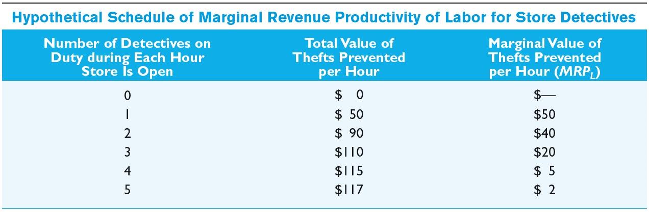
5 3.2 The Short-Run Demand for Labor When Both Product and Labor Markets Are Competitive In the short-run, the firm cannot vary its stock of capital, therefore, the production function takes the form: Q f ( L, K) This means the firm needs only to decide whether to alter its output level; how to increase or decrease output is not an issue, because only the employment of labor (L) can be adjusted see Table 3.1

6 Table 3.1

7 3.2 The Short-Run Demand for Labor When Both Product and Labor Markets Are Competitive When both product and labor markets are competitive, it is assumed that: All producers or sellers are price takers in the product market. All employers of labor are wage takers in the labor market. Analysis of a firm s production and employment is in the short run where the firm cannot vary its capital stock. With short production, only the employment of labor can be adjusted.

8 3.2 The Short-Run Demand for Labor When Both Product and Labor Markets Are Competitive A Critical Assumption: Declining MP L Since K is constant in the short-run, adding extra unit of L increases output in each case MP L is positive to some point. Eventually, adding more L will produce progressively smaller increments of output law of diminishing marginal returns. This means that as employment expands, each additional worker has a progressively smaller share of the capital stock to work with.

9 3.2 The Short-Run Demand for Labor When Both Product and Labor Markets Are Competitive From Profit Maximization to Labor Demand Profits are maximized only when employment is such that any further one-unit change in labor would have a marginal revenue product equal to marginal expense: MRP L = ME L (3.4) MP L. P = W (3.5) MP L = W/P (3.6)

10 3.2 The Short-Run Demand for Labor When Both Product and Labor Markets Are Competitive Labor Demand in Terms of Real Wages Labor demand can be analyzed in terms of either real or money wages. The negative slope of the labor demand curve indicates that each additional unit of labor employed produces a progressively smaller increment in output. At any real wage determined by the market, the firm should employ labor up to the point at which MP L equals the real wage (W/P) the firm s demand for labor in the short-run is equivalent to the downward-sloping segment of its MP L schedule: At E 0 employment level: MP L = W/P profit maximizing level of employment. At E 1 employment level: MP L > W/P employment level E 1 is less than E 0 ; firm could increase profit by adding L. At E 2 employment level: MP L < W/P employment level E 2 is greater than E 0 ; firm could increase profit by decreasing L.

11 Figure 3.1 Demand for Labor in the Short Run (Real Wage)

12 3.2 The Short-Run Demand for Labor When Both Product and Labor Markets Are Competitive Labor Demand in Terms of Money Wages In some circumstances, labor demand curves are more readily conceptualized as downward-sloping functions of money wages. MRP L does not decline because added workers are incompetent, it declines because capital stock is fixed, hence added workers have less capital or equipment to work with. The fundamental point is: the labor demand curve in the short-run slopes downward because it is the MRP L curve, which slopes downward because of labor s diminishing marginal product. Since MRP L = W for a profit maximizer who takes wages as given, the MRP L curve and labor demand curve (MP L ) must be the same. The marginal product of an individual is not a function solely of his or her personal characteristics: It depends on the number of similar employees hired by the firm and the firm s capital stock.

13 Table 3.2

14 Figure 3.2 Demand for Labor in the Short Run (Money Wage)

15 3.2 The Short-Run Demand for Labor When Both Product and Labor Markets Are Competitive Market Demand Curves A market demand curve (or schedule) is the summation of the labor demanded by all firms in a particular labor market at each level of the real wage When real wage changes (falls or increases), the number of workers that existing firms want to employ changes (increases or falls) Objections to the Marginal Productivity Theory of Demand Employers do not go around verbalizing MRP L it is a theoretical concept, which assumes a degree of sophistication that most employers do not have With fixed capital stock, it seems that adding labor would not add to output at all but workers take their turns in using the fixed capital stock such that labor will generally have a marginal product greater than zero

16 3.3 The Demand for Labor in Competitive Markets When Other Inputs Can be Varied Labor Demand in the Long Run In long-run, the firm s ability to adjust other inputs such as capital will affect the demand for labor To maximize profits in the long-run, the firm must adjust L and K such that each input s MRP is equal to its ME MP L.P = W (a restatement of equation 3.5) (3.7a) MP K.P = C (the profit maximizing condition for K) Rearranging equations (3.7a) and (3.7b) yields: P = W/MP L P = C/MP K W/MP L = C/MP K (3.7b) (3.8a) (3.8b) (3.8c)

17 3.3 The Demand for Labor in Competitive Markets When Other Inputs Can be Varied W is the added cost or marginal cost (MC) of producing MPL an added unit of output when using labor to generate the increase in output C is the marginal cost (MC) of producing an extra unit MPK of output when using capital to generate the increase in output To maximize profits, the firm must adjust its labor and capital inputs so that the marginal cost of producing an added unit of output using labor is equal to the marginal cost of producing an added unit of output using capital

18 3.3 The Demand for Labor in Competitive Markets When Other Inputs Can be Varied W MP Given = in equation (3.8c), if W increases: L Adjustment will have to be made to the use of labor (L). The firm will have to cut back on the use of L, which will raise its MP L. Each unit of capital (K) has less labor (L) working with it, therefore, MP K falls and the firm s profit-maximizing level of level output will fall scale effect. W MP Since > and if L given an W, the MP L and the L C MP K C MP K MP K will adjust to restore =. The rise in W can also cause the firm to change its input mix by substituting capital for labor substitution effect. W MP L C MP K

19 3.3 The Demand for Labor in Competitive Markets When Other Inputs Can be Varied More Than Two Inputs Capital and labor are not the only inputs used in the production process. Labor can be subdivided into many categories by age, educational level, and occupation. Other inputs in the production process include materials and energy. For all other inputs, the equality of MC in using these inputs to produce an added unit of output as given by equation (3.8c) applies.

20 3.3 The Demand for Labor in Competitive Markets When Other Inputs Can be Varied If Inputs Are Substitute in Production If two inputs are substitutes in production, and if an increase in the price of one input shifts the demand for another input to the left as in panel (a) of Figure 3.3, then the scale effect dominates the substitution effect inputs are gross complements. If the increase in the price of one input shifts the demand for the other input to the right as indicated in panel (b) of Figure 3.3, then the substitution effect dominates inputs are gross substitutes. If Inputs Are Complements in Production When two inputs must be used together in some proportion, they are considered to be perfect complements or complements in production that is, no substitution effect, only scale effect.

21 Figure 3.3 Effect of Increase in the Price of One Input (k) on Demand for Another Input (j), Where Inputs Are Substitutes in Production

22 3.4 Labor Demand When the Product Market Is Not Competitive Monopoly producers are price-makers in the product market but wage-takers in the labor market. They use MRP L = ME L to determine the profit-maximizing level of employment. Maximizing Monopoly Profits To maximize monopoly profits, a monopolist will hire until: MRP L = MR.MP L = W (3.9) Dividing both sides by P (recall that P > MR) yields: MR P. MPL W P (3.10)

23 3.4 Labor Demand When the Product Market Is Not Competitive Do Monopolies Pay Higher Wages? Economists suspect that product-market monopolies pay wages that are higher than what a competitive firms would pay and pass the costs along to consumers in the form of higher prices. The ability to pay higher wages makes it possible for managers to hire people who might be more attractive or personable or have other characteristics managers find desirable.

24 3.5 Policy Application: The Labor Market Effects of Employer Payroll Taxes and Wage Subsidies Governments finance certain social programs through taxes payroll taxes that require employers to remit payments based on their total payroll costs. Who Bears the Burden of a Payroll Tax? Payroll taxes are used to finance government programs such as: Unemployment insurance Social Security retirement Disability Medicare/Medicaid Let X be the fixed amount of tax per labor hour rather than a percentage of payroll.

25 3.5 Policy Application: The Labor Market Effects of Employer Payroll Taxes and Wage Subsidies Shifting the Demand Curve Payroll taxes will shift the labor demand curve to the left. Employers will decrease their employment of workers if their wage costs (wage bill) increase by the tax amount of X (that is, W + X ) due to payroll tax. Employers will retain the same amount of workers as before the payroll tax was imposed if the entire tax burden is passed onto the workers, that is, workers wages fall by the tax amount of X (hence, W X). Employees bear a burden in the form of lower wage rates and lower employment levels when the government chooses to generate revenues through a payroll tax on employers.

26 Figure 3.4 The Market Demand Curve and Effects of an Employer-Financed Payroll Tax

27 3.5 Policy Application: The Labor Market Effects of Employer Payroll Taxes and Wage Subsidies Effects of Labor Supply Curves If the labor supply curve were vertical meaning that lower or higher wages have no effect on labor supply the entire amount of the tax will be shifted to workers in the form of a decrease in their wages by the amount of X (hence W X). The incidence of tax burden on employers and employees depends on the responsiveness (elasticities) of labor demand and labor supply to changes in wages. If wages do not fall due to an employer payroll-tax increase, employment levels will, and employer labor costs will increase thus reducing the quantity of labor demanded.

28 Figure 3.5 Payroll Tax with a Vertical Supply Curve

29 3.5 Policy Application: The Labor Market Effects of Employer Payroll Taxes and Wage Subsidies Employment Subsidies as a Device to Help the Poor Government subsidies of employers payroll could be in different forms: Cash payments Tax credit to employers Target Job Tax Credit (TJTC), General or selective/targeted. Let X be the fixed amount of subsidy that the government paid the employer per labor hour. Subsidies shift the labor demand curve to the right, thus creating pressures to increase employment levels and the wages received by employees.

30 MODERN LABOR ECONOMICS THEORY AND PUBLIC POLICY 12 TH EDITION CHAPTER 3A Graphical Derivation of a Firm s Labor Demand Curve

31 The Production Function Figure 3A.1: A Production Function Q = f (L, K)

32 The Slope of the Isoquant Along any isoquant, K can be decreased for much larger increase in L, but Q will remain unchanged That is, labor could be substituted for capital to maintain a given level of production (ΔQ = 0): Q Q ΔK.MP K + ΔL.MP L = 0 = K. L. K L Q Q ΔK.MP K = ΔL.MP L or K. L. K L MP MP L K K L MRTS K L Q (3.A1)

33 Demand for Labor in the Short Run Earlier in the Chapter, we assumed that capital is fixed in the short-run hence Q f ( L, K) and that labor is hired until labor s MP L = W/P Holding capital constant at K a, the firm can produce: Q = 100 by employing L a workers Q = 150 by employing L a workers Q = 200 by employing L a workers The extra labor (L a L a ) required to produce 50 units of added output is greater than the extra labor (L a L a ) that produced the first 50-unit increment see Figure 3A.2. The assumptions that MP L declines as employment is increased and that firms hire until MP L = W/P are the bases for the assertion that a firm s short-run demand curve for labor slopes downward.

34 Figure 3A.2 The Declining Marginal Productivity of Labor

35 Demand for Labor in the Long Run Recall that a firm maximizes its profits by producing at a level of output (Q*) where MC = MR. For a competitive firm, MR is equal to output/product price, that is, P = MR. Conditions for Cost Minimization How will the firm combine labor and capital to produce the Q*? Profit maximization is possible if Q* is produced using the least expensive method. Cost of producing Q* can be given by three isoexpenditure lines: Line AA : 20K + 10L = 1,000 Line BB : 20K + 10L = 1,500 Line DD : 20K + 10L = 2,000

36 Figure 3A.3 Cost Minimization in the Production of Q* (Wage = $10 per Hour; Price of a Unit of Capital = $20)

37 The MRTS as defined in equation (3A.1) can be rewritten as: Rearranging, Slope of the isoexpenditure line is:. At the cost minimizing point: Since MRTS is K/ Q MRTS L/ Q K / Q Q / L MP MRTS L / Q Q / K MP K L MRTS this version of the MRTS to : / / Q Q MP MP (3A.2) (3A.3) [a rearranged version of equation (3.8c)] (see equation 3A.2) and equating W C W C 20 L K L K W C (3A.4) K / Q W L / Q C (3A.5) K L. C. W Q Q (3A.6)

38 The Substitution Effect Isoexpenditure line BB shows the cost minimizing point in producing Q* where the wage rate is $10 and the rental cost of capital is $20, which remained constant when the wage rate increased to $20 (doubled). W to $20 rotates the isoexpenditure line BB inward to BB and it is no longer tangent to isoquant Q*, that is, Q* can no longer be produced for $1,500. It is assumed that the least-cost expenditure to produce Q* increases to $2,250 and EE is the new isoexpenditure line. The increased labor cost will induce the firm to substitute capital for labor see point Z in Figure 3A.4. The reduction in employment from L Z to L Z is the substitution effect generated by the wage increase.

39 Figure 3A.4 Cost Minimization in the Production of Q* (Wage = $20 per Hour; Price of a Unit of Capital = $20)

40 The Scale Effect Suppose that the profit-maximizing level of output falls from Q* to Q** and that all isoexpenditure lines have a new slope of 1 when W = $20 and C = $20 see Figure 3A.5. The cost-minimizing way to produce Q** is at Z where the isoexpenditure line FF is tangent to the Q** isoquant. The overall response in employment of labor due to the increase in the wage rate is the fall in labor usage from L Z to L Z. Recall that the decline from L Z to L Z is know as the substitution effect due to a wage change. The scale effect is the reduction in employment from L Z to L Z reduction in the usage of both K (at K Z not shown) and L (at L Z ) because of the reduced scale of production.

41 Figure 3A.5 The Substitution and Scale Effects of a Wage Increase

42 Labor Supply Outline Trends in Labor Force Participation and Hours of Work Labor Force Participation Rates Hours of Work A Theory of the Decision to Work Some Basic Concepts Analysis of the Labor/Leisure Choice Empirical Findings on the Income and Substitution Effects Policy Application Budget Constraints with Spikes Programs with Net Wage Rates of Zero Subsidy Programs with Positive Net Wage Rates

43 6.1 Trends in Labor Force Participation and Hours of Work Recall from Chapter 2 that: LFPR LF x100 WAP Labor Force Participation Rates Over the past ten decades, LFPR Women more than doubled while the LFPR Men decreased due to a host of factors. Similar trends have been observed in other advanced countries Canada, France, Germany, Japan, and Sweden Hours of Work Initially, American workers worked 55 hours per week, but that has declined to less than 40 hours per week.

44 6.2 A Theory of the Decision to Work Labor is the most abundant and important factor of production, therefore, a country s economic performance depends on the willingness of its people to work. A person s discretionary time (16 hours a day) can be spent: (a) working for pay to derive income (Y ) for consumption, and (b) on leisure (L). Some Basic Concepts Recall that the demand for good/service depends on: (1) The opportunity cost of the good = market price (2) One s level of wealth (3) One s set of preferences

45 6.2 A Theory of the Decision to Work Opportunity Cost of Leisure - The demand for leisure depends on: The opportunity cost of leisure, which is equal to one s wage rate or the extra earnings a worker can take home from an extra hour of work. Wealth and Income Wealth and income include: (a) family s holdings of bank accounts (b) financial investments (c) physical property or properties The effects of increases in income and wages on leisure-work preferences of a person can be categorized as: (1) Income effect (2) Substitution effect

46 6.2 A Theory of the Decision to Work Defining the Income Effect If income increases, holding wages constant, desired hours of work will go down demand for leisure hours will increase while the hours of work supplied by a worker to the labor market decreases. That is: H Income Effect W 0 (6.1) Y Defining the Substitution Effect If income is held constant, an increase in the wage rate will raise the price and reduce the demand for leisure, thereby increasing work incentives an increase in the opportunity cost of leisure reduces the demand for leisure. That is: H Substitution Effect Y 0 (6.2) W

47 6.2 A Theory of the Decision to Work Observing Income and Substitution Effects Separately It is possible to observe situations or programs that create only one effect or the other receiving an inheritance is an example of the income effect, which induces the person to consume more leisure, thus reducing the willingness to work. Both Effects Occur When Wages Rise The labor supply response to a simple wage increase will involve both an income effect and a substitution effect; and both effects working in opposite directions creates ambiguity in predicting the overall labor supply response in many cases see Figure 6.1, p.178. If the income effect is stronger, the person will respond to a wage increase by decreasing his or her labor supply the labor supply curve will be negatively sloped that is, as W H. If the substitution effect dominates, the person s labor supply curve will be positively sloped that is, as W H.

48 Figure 6.1 An Individual Labor Supply Curve Can Bend Backward

49 6.2 A Theory of the Decision to Work Analysis of the Labor/Leisure Choice The theory of labor supply is easier to understand by using the concept of indifference curves and budget constraints. Preferences U = f (Y, L), where U is an index that measures the level of satisfaction or happiness, Y is income (wage) and L is leisure. Higher U means higher levels of utility that will make a person happier. Along the indifference curve: Y. MU L. MU 0 Y MU L Y MU L or L MU L MU Y Y Y MRS YL, L

50 6.2 A Theory of the Decision to Work Indifference curves show the various combinations of money income (or goods and services) and the hours of leisure/work per day that will yield the same level of happiness. Characteristics of the indifference curves: (1) Consumer preferences are usually northeast on the higher or highest indifference curve see Figure 6.2. (2) Indifference curves do not intersect. (3) Indifference curves are negatively sloped see Figure 6.3. (4) Indifference curves are convex steeper at the left than at the right when income is high, leisure hours are relatively few. (5) Moving down on the indifference curve reflects value when income is low, leisure hours are abundant see Figure 6.3. (6) Indifference curves differ among individuals because of the differences in tastes/preferences or values see Figure 6.4.

51 Figure 6.2 Two Indifference Curves for the Same Person (Y ) (L)

52 Figure 6.3 An Indifference Curve

53 Figure 6.4 Indifference Curves for Two Different People

54 6.2 A Theory of the Decision to Work Income and Wage Constraints Budget constraints show the combinations of money income (or attainable consumption goods and services) and the hours of leisure per day that are possible or attainable for the individual. For simplification: Let V = nonlabor income (property income, inheritances, lottery winnings, dividends,) see line Dd in Figure 6.7 H = number of hours allocated to the labor market w = hourly wage rate L = hours of leisure per day Y = total income defined as: Y = wh + V Y = wh (if nonlabor income is zero, that is V = 0) T = total discretionary time (16 hours) T = H + L

55 6.2 A Theory of the Decision to Work That is, Y = w(t L) + V or Y = (wt + V) wl see line ED in Figure 6.5 The slope of the constraint can be expressed as: Y L w Y w H Y Wage Rate (6.3) H

56 Figure 6.5 Indifference Curves and Budget Constraint (Y ) At point N: Y L L or MU MU Y w MRS Y, L w ( L ) (H )

57 Figure 6.6 The Decision Not to Work Is a Corner Solution This diagram shows that the preference for leisure is so strong, hence there is no desire to work at all in the labor market. That is, H = 0 and L = 16 at point D.

58 6.2 A Theory of the Decision to Work The Income Effect Property income, inheritances, lottery prizes, and dividends are nonlabor incomes that shift the budget constraint upward holding the wage rate (W) constant. An income effect would be observed if nonlabor income increased and the person supplied 0 hours of work to the labor market. The new source of income (holding the wage rate constant) can cause the worker to supply less hours of work per day and take more hours of leisure. - see Figure 6.7, p. 185.

59 Figure 6.7 Indifference Curves and Budget Constraint (with an Increase in Nonlabor Income) If V (line Dd), and W is held constant, this would result in H and L. The income effect dominates hence the move from point N to point P on a higher Utility Level B.

60 6.2 A Theory of the Decision to Work Income and Substitution Effects with a Wage Increase If nonlabor income is zero or unchanged (that is, holding wealth constant) and the wage rate (W ) increased, this would cause both an income effect and a substitution effect: If due to W, a worker increases his or her hours of work to the labor market, then the substitution effect is stronger than the income effect see Figure 6.8, p If due to W, a worker reduces his or her hours of work to the labor market, then the income effect is stronger than the substitution effect see Figure 6.9, p The difference between the substitution effect and income effect of a wage increase lies solely in the shape of the indifference curves.

61 Figure 6.8 Wage Increase with Substitution Effect Dominating When W, this leads to H and L, and the substitution effect dominates, hence the move from point N 1 to point N 2 on a higher level of utility given by U 2.

62 Figure 6.9 Wage Increase with Income Effect Dominating A W leads to H (from 8 to 6 hours) and L (from 8 to 10 hours), and the income effect dominates.

63 6.2 A Theory of the Decision to Work Isolating Income and Substitution Effects Remember that any given wage increase (W ) can raise a worker s utility level (e.g. from U 1 to U 2 ) and thus induce: H and L substitution effect. H and L income effect. The hypothetical question is: What would have been the change in labor supply if the worker reached a new (higher) indifference curve with a V instead of a W? The budget constraint will shift northeast parallel to the old budget constraint, holding W constant. The worker attains higher level of utility with reduced work hours associated with greater wealth at the new point of tangency. An W (holding wealth constant) causes a worker to end on a higher portion of the same indifferences with H and L.

64 Figure 6.10 Wage Increase with Substitution Effect Dominating: Isolating Income and Substitution Effects A wage increase, with V constant, raises the level of utility to U 2 and induces more hours of work from 8 to 11 hours per day. If the wage increase is, instead, replaced by an increase in nonlabor income (V), with W constant, a higher level of utility is attained at point N 3 on U 2 with H and L. With a wage change, the person is induced to work 11 hours per day at point N 2 on utility level U 2. Without the W, and U constant at U 2, the person would have chosen to work 7 hours per day at point N 3.

65 6.2 A Theory of the Decision to Work Which Effect Is Stronger The extent of the income effect and substitution effect of a wage increase depends on the slopes of the indifference curves and the new budget constraints. If the worker had a relatively flat set of difference curves, the initial tangency might imply a relatively heavy work schedule. If the person had more steeply sloped difference curves, the initial tangency might imply that hours at work are fewer. Other things equal, people who are working longer hours will exhibit greater income effects when wage rates change.

66 6.2 A Theory of the Decision to Work For someone depicted by the indifference curve A and the budget line DE in Figure 6.6, he/she was initially out of the labor force, and his/her utility was maximized at point D same as point C given constraint CD in Figure A wage increase (see Figure 6.6 and Figure 6.11) can induce two outcomes: The person will either begin to work for pay or remain out of the labor force. Reducing the hours of paid employment is not possible. A dominant substitution effect will occur: If a wage increase induces the decision to participate. If a wage fall causes someone to drop out of the labor force. The labor force participation decisions brought about by wage changes exhibit a dominant substitution effect.

67 Figure 6.11 The Size of the Income Effect Is Affected by the Initial Hours of Work A W changes the budget line CD to CE. With flatter U curves, the point of tangency will occur at point A with H and L. With steeper U curves, the point of tangency will occur at point B with less H and more L. Note that a person at point C is not in the labor force because the wage (W CD ) slope of line CD may be lower than what will induce labor market participation.

68 6.2 A Theory of the Decision to Work The Reservation Wage A worker takes into consideration some key factors in determining whether or not to work in the labor market: Reservation wage and the earning possibilities. Commute time per day (fixed costs of working) see Figure A reservation wage (W R ) is the wage below which a person will not work in the labor market that is, W R represents the value placed on an hour of lost leisure time. Often, people are thought to behave as if they have both a reservation wage and a certain number of work hours that must be offered before the consideration to take a job.

69 Figure 6.12 Reservation Wage with Fixed Time Costs of Working Line segment AB = Fixed time costs of commute. Let the slope of budget line BC = W BC. Let the slope of budget line BD = W BD and W BC < W BD. If W BC < W R This person will not work at all. If W BD W R This person will work at least 4 hours and will take 10 hours of leisure per day.

70 6.2 A Theory of the Decision to Work Empirical Findings on the Income and Substitution Effects Labor supply theory suggests that the choices workers make with respect to the desired hours of work depends on: Wealth Wage rate Leisure-income preferences A comprehensive review of numerous studies of the labor supply of men finds that the sizes of the estimated effects vary with both data and the statistical methodology used. Overall, the observed substitution effects are positive while the observed income effects are negative. Studies of the labor supply behavior of women generally have found a greater responsiveness to wage changes than is found among men.

71 6.3 Policy Applications We use labor supply theory to analyze the work-incentive effects of various social or income maintenance programs because they create budget constraints for their recipients. Budget Constraints with Spikes The social insurance compensation programs compensate workers for work-related injuries replaces most of the earnings/incomes lost by workers due to injuries. Compensations are paid as long as the worker is off work and disabled, and payments cease even if the worker supplies only one hour of labor. These programs affect the work-incentives of workers since the returns associated with the first hour of work are negative reduced income for returning to work for 1 hour.

72 Figure 6.13 Budget Constraint with a Spike Pre-injury budget line AB W AB with earnings given as E 0 (= AC) at point f where H = 8 and L = 8. With compensation for injury, the post-injury budget constraint is BAC with AC as the spike. The worker will be happy to be at point C on a higher level of utility where H = 0 and L = 16, more so, since the no-work pay given by AC is equal to E 0 the pre-injury pay at point f where H = 8 and L = 8. The income effect raises a worker s W R (slope of the dashed line > W AB ) hence this slows his or her return to work.

73 6.3 Policy Applications Since income maintenance programs create spikes and severe work disincentive problems: What can policymakers do to minimize the effects? Set no-work benefits at some fraction of pre-injury earnings. Set benefits at Ag (see Figure 6.13 ) so that a worker is on his or her pre-injury indifference but with earnings less than E 0 or set benefits slightly less than Ag (about half the preinjury earnings) so that a worker will be eager to return to work as soon as he or she is physically able to do so. Set an upper limit on the weeks each unemployed worker can receive the no-work benefits. If extensions are to be granted in some cases, set up a panel medial or judicial board to review such cases.

74 6.3 Policy Applications Programs with Net Wage Rates of Zero Other social welfare programs have different eligibility criteria and calculate benefits differently. Program benefits are paid based on the difference between one s actual earnings (Y a ) and one s needs (Y n ). Payment of benefits based on the difference between actual earnings and needs creates a net wage rate of zero. Nature of Welfare Subsidies The welfare agency determined the income needed (Y n ) by an eligible person based on: family size, area living costs CPI, and local welfare regulations.

75 6.3 Policy Applications For subsidy recipients, an extra hour of work yielded no net increase in income, because the extra earnings resulted in an equal reduction in welfare benefits price of leisure was zero see the slope of line BC in Figure A welfare program that increases the income of the poor creates an income effect which tends to reduce labor supply as it also causes the wage to effectively drop to zero because every dollar earned is matched by a dollar reduction in welfare benefits. The dollar-for-dollar reduction in benefits induces a huge substitution effect, which causes welfare recipients to reduce their hours of hour to zero at point B see Figure 6.14.

76 Figure 6.14 Income and Substitution Effects for the Basic Welfare System Let a worker s actual earnings = Y a (at point E) and his or her income needs = Y n. Paying the difference between Y a and Y n yields a net wage rate of zero (slope of line BC). Payment to the individual = Y n Y a, and if Y a = 0 because H = 0, s/he receives a subsidy of Y n. If H > 0, earnings cause $-for-$ reductions in welfare benefits which create budget line ABCD.

77 Figure 6.15 The Basic Welfare System: A Person Not Choosing Welfare If a worker s indifference curves were sufficiently flat so that the curve tangent to segment CD passed above point B, this worker s utility would be maximized by choosing to work instead of receiving welfare at point B this is lower in comparison to point B shown in Figure 6.14.

78 6.3 Policy Applications Welfare Reform The United States made/adopted major changes to its income-subsidy programs in the 1990s because of the work disincentives inherent in the traditional welfare programs. The Personal Responsibility and Work Opportunities Reconciliation Act (PRWORA) gave states more authority on how to design their own welfare programs: (1) encourage work, (2) reduce poverty, and (3) move people off welfare. These changes appeared to have increased the LFPR of single mothers from 68% in 1994 to 78% in 2000.

79 6.3 Policy Applications Lifetime Limits PRWORA placed a five-year lifetime limit on recipients: Reduce how long families could be on welfare. Increase work incentives by eliminating income subsidy. Potential welfare recipients must choose when to receive the subsidy and when to save their eligibility in the event of a future need. Work Requirements PRWORA of 1996 introduced a work requirement into the welfare system by requiring 6 hours of work per day (or at least 30 hours per week) after a recipient has been on welfare for two years. Enrollment in education and training programs count toward work requirement see Figures 6.16 and The work-incentive effects of the work requirement will depend on whether the indifference curves are steeply sloped or flatly sloped.

80 Figure 6.16 The Welfare System with a Work Requirement Work requirement = 6 hours per day (or 30 hours per week). If a person fails to work the 6 hours per day as required, no welfare benefits will be received. If earnings from 6 hours of work requirement are less than Y n, then welfare benefits will be received (given by line segment BCD). If work requirement is exceeded, income remains at Y n and the welfare recipient will be along line CD, but if earnings rise above Y n and he/she is along line DE, he/she will no longer be eligible for welfare.

81 6.3 Policy Applications Subsidy Programs with Positive Net Wage Rates The PRWORA and Earned Income Tax Credit (EITC) are income maintenance programs designed by the federal government: PRWORA creates positive net wages. EITC functions as an earnings (cash) subsidy, which goes only to those who work. The tax credit offered by the EITC programs varies with one s earnings and the number of dependent children. EITC recipients could experience: Income effect that pushes them in the direction of less work those whose annual income falls between $13,090 and $41,952. Substitution effect that pushes the recipients in the direction of more work, thus the labor force participation of low-income workers will increase those whose annual income is less than $13,090.

82 Figure 6.17 Earned Income Tax Credit (Unmarried, Two Children), 2012 The EITC as an earnings subsidy creates a budget constraint of ABDEC. For workers with earnings of $13,090 or less, the tax credit is 40% of earnings, and the maximum tax credit allowed for a single parent with two children was $5,236 in Incomes between $13,090 and $17,100 qualify for the maximum tax credit: Line AB = $18,326 Line AD = $22,336. Earnings of $41,952 and above do not qualify for this tax credit.