A Multiplicative Seasonal Box-Jenkins Model to Nigerian Stock Prices

Transcription

1 A Multiplicative Seasonal Box-Jenkins Model to Nigerian Stock Prices Ette Harrison Etuk Department of Mathematics/Computer Science, Rivers State University of Science and Technology, Nigeria ABSTRACT Time series analysis of Nigerian Stock Prices Data is done. The data used is monthly from 1987 to The time plot reveals a negative trend and no clear seasonality. A multiplicative seasonal model is suggestive given seasonality that tends to increase with time. Seasonal differencing once produced a series with a slightly positive trend but still with no discernible stationarity. A non-seasonal differencing of the seasonal differences yielded a series with no trend but with a correlogram revealing stationarity of order 12 and a seasonal moving average component. A multiplicative seasonal autoregressive integrated moving average (ARIMA) model, (0, 1, 1)x(0, 1, 1) 12, is fitted to the series. Keywords: Stock Prices, Seasonal Time Series, ARIMA model, Nigeria 1. INTRODUCTION A time series is defined as a set of data collected sequentially in time. It has the property that neighbouring values are correlated. This tendency is called autocorrelation. A time series is said to be stationary if it has a constant mean and variance. Moreover the autocorrelation is a function of the lag separating the correlated values and called the autocorrelation function (ACF). A stationary time series {X t } is said to follow an autoregressive moving average model of orders p and q (designated ARMA(p, q)) if it satisfies the following difference equation Or X t - 1 X t-1-2 X t p X t-p = t + 1 t t q t-q (1) A(L)X t = B(L) t (2) where { t }is a sequence of uncorrelated random variables with zero mean and constant variance, called a white noise process, and the i s and j s constants; A(L) = 1-1 L - 2 L p L p and B(L) = L + 2 L q L q and L the backward shift operator defined by L k X t = X t-k. If p = 0, the model (1) becomes a moving average model of order q (designated MA(q)). If, however, q = 0 it becomes an autoregressive process of order p (designated AR(p)). An AR(p) model may be defined as a model whereby a current value of the time series X t depends on the immediate past p values: X t-1, X t-2,, X t-p. On the other hand an MA(q) model is such that the current value X t is a linear combination of immediate past values of the white noise process: t-1, t-2,, t-q. Apart from stationarity, invertibility is another important requirement for a time series. It refers to the property whereby the covariance structure of the series is unique (Priestley, 1981). Moreover it allows for meaningful association of current events with past history of the series (Box and Jenkins, 1976). An AR(p) model may be more specifically written as X t + p1 X t-1 + p2 X t pp X t-p = t Then the sequence of the last coefficients { ii } is called the partial autocorrelation function (PACF) of {Xt}. The ACF of an MA(q) model cuts off after lag q whereas that of an AR(p) model is a combination of sinusoidals dying off slowly. On the other hand the PACF of an MA(q) model dies off slowly whereas that of an AR(p) model cuts off after lag p. AR and MA models are known to exhibit some duality relationships. These include: 1. A finite order AR model is equivalent to an infinite order MA model. 2. A finite order MA model is equivalent to an infinite order AR model. 1

2 3. The ACF of an AR model exhibits the same behaviour as the PACF of an MA model. 4. The PACF of an AR model exhibits the same behaviour as the ACF of an MA model. 5. An AR model is always invertible but is stationary if A(L) = 0 has zeros outside the unit circle. 6. An MA model is always stationary but is invertible if B(L) = 0 has zeros outside the unit circle. Parametric parsimony consideration in model building entails preference for the mixed ARMA fit to either the pure AR or the pure MA fit. Stationarity and invertibility conditions for model (1) or (2) are that the equations A(L) = 0 and B(L) = 0 should have roots outside the unit circle respectively. Often, in practice, a time series is non-stationary. Box and Jenkins (1976) proposed that differencing of appropriate order could render a non-stationary series {Xt} stationary. Let degree of differencing necessary for stationarity be d. Such a series {Xt} may be modeled as A(L) d X t = B(L) t (3) where = 1 - L and in which case A(L) d = 0 shall have unit roots d times. Then differencing to degree d renders the series stationary.the model (3) is said to be an autoregressive integrated moving average model of orders p, d and q and designated ARIMA(p, d, q). 2. SEASONAL ARIMA MODELS A time series is said to be seasonal of order d if there exists a tendency for the series to exhibit periodic behaviour after every time interval d. Traditional time series methods involve the identification, unscrambling and estimation of the traditional components: secular trend, seasonal component, cyclical component and the irregular movement. For forecasting purpose, they are reintegrated. Such techniques could be quite misleading. The time series {X t } is said to follow a multiplicative (p, d, q)x(p, D, Q) s seasonal ARIMA model if A(L) (L s ) d D sx t = B(L) (B s ) t (4) where and are polynomials of order P and Q respectively. That is, (L s ) = L s + + P L sp (5) (L s ) = L s + + q L sq (6) where the i and the j are constants such that the zeros of the equations (5) and (6) are all outside the unit circle for stationarity or invertibility respectively. Equation (5) represents the autoregressive operator whereas (6) represents the moving average operator. Existence of a seasonal nature is often evident from the time plot. Moreover for a seasonal series the ACF or correlogram exhibits a spike at the seasonal lag. Box and Jenkins (1976) and Madsen (2008) are a few authors that have written extensively on such models. A knowledge of the theoretical properties of the models provides basis for their identification and estimation. The purpose of this paper is to fit a seasonal ARIMA model to the Nigerian Stock Prices (NSP). 3. MATERIALS AND METHODS The data for this work are monthly Stock Prices from 1987 to 2006 obtainable from the Nigerian Stock Exchange Office, Port Harcourt, Nigeria Determination of the orders d, D, P, q and Q: Seasonal differencing is necessary to remove the seasonal trend. If there is secular trend non-seasonal differencing will be necessary. To avoid undue model complexity it has been advised that orders of differencing d and D should add up to at most 2 (i.e. d + D < 3). If the ACF of the differenced series has a positive spike at the seasonal lag then a seasonal AR component is suggestive; if it has a negative spike then a seasonal MA term is suggestive 2

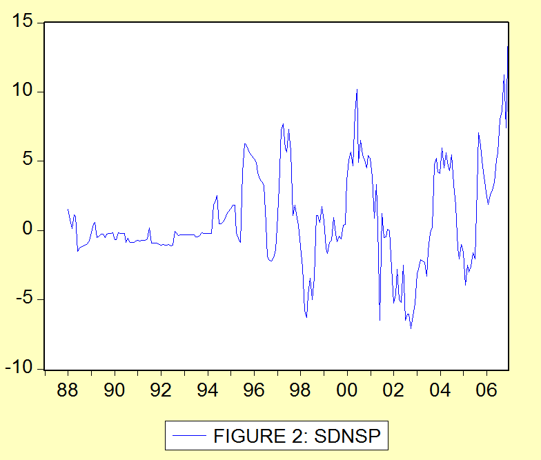
3 As already mentioned above, an AR(p) model has a PACF that truncates at lag p and an MA(q) has an ACF that truncates at lag q. In practice 2/ n where n is the sample size are the non-significance limits for both functions Model Estimation The involvement of the white noise process in an ARIMA model entails a nonlinear iterative process in the estimation of the parameters. An optimization criterion like least error sum of squares, maximum likelihood or maximum entropy is used. An initial estimate is usually used. Each iteration is expected to be an improvement of the last one until the estimate converges to an optimal one. However, for pure AR and pure MA models linear optimization techniques exist (See for example, Box and Jenkins(1976), Oyetunji(1985)). There are attempts to adopt linear methods to estimate ARMA models (See for example, Etuk(1987, 1998)). We shall use Eviews software which employs the least squares approach involving nonlinear iterative techniques Diagnostic Checking The model that is fitted to the data should be tested for goodness-of-fit. We shall do some analysis of the residuals of the model. If the model is correct, the residuals would be uncorrelated and would follow a normal distribution with mean zero and constant variance. The autocorrelations of the residuals should not be significantly different from zero. 4. RESULTS AND DISCUSSION The time plot of the original series NSP in Figure 1 shows a slightly positive trend and no clear seasonality. However the seasonality increases with time indicating a multiplicative seasonal model. Seasonal (i.e. 12- month) differencing of the series produces a series SDNSP with a slightly positive trend but with no clear seasonality (see Figure 2). Non-seasonal differencing of SDNSP yields a series DSDNSP with no trend and no clear seasonality (See Figure 3). However, its ACF in Figure 4 has a negative spike at lag 12 revealing a seasonality of lag 12 and a seasonal MA component of order one to the model. We propose the (0, 1, 1)x(0, 1, 1) 12 model DSDNSP t = 1 t t t-13 (7) The model as summarized in Table 1 is given by DSDNSP t = t t t-13 + t (8) ( ) ( ) ( ) The estimation involved 28 iterations. Only the last two coefficients are significantly different from zero, each being larger than twice its standard error. The correlogram of the residuals in Figure 5 depicts the adequacy of the model. Virtually all the residual autocorrelations are not significantly different from zero. Moreover the histogram of the residuals in Figure 6 shows that they are normally distributed with zero mean further indicating model adequacy. 5. CONCLUSION We conclude that Nigerian Stock Price Data follow an adequate (0, 1, 1)x(0, 1, 1) 12 model. REFERENCES 1. Box, G. E. P. and Jenkins, G. M. (1976). Time Series Analysis, Forecasting and Control, Holden-Day, San Francisco. 2. Etuk, E. H. (1987). On the Selection of Autoregressive Moving Average Models. An unpublished Ph. D. Thesis, Department of Statistics, University of Ibadan, Nigeria. 3. Etuk, E. H. (1998). An Autoregressive Integrated Moving Average (ARIMA) Simulation Model: A Case Study. Discovery and Innovation, Volume 10, Nos. 1 & 2: pp Madsen, H. (2008). Time Series Analysis, Chapman & Hall/CRC, London. 5. Oyetunji, O. B. (1985). Inverse Autocorrelations and Moving Average Time Series Modelling. Journal of Official Statistics, Volume : pp Priestley, M. B. (1981). Spectral Analysis and Time Series. Academic Press, London. 3

4 4

5 FIGURE 4: CORRELOGRAM OF DSDNSP 5

6 TABLE 1: MODEL ESTIMATION FIGURE 5: CORRELOGRAM OF RESIDUALS 6

7 FIGURE 6: HISTOGRAM OF RESIDUALS 7