The Solow Model. Zongye Huang 1. Dec, Capital University of Economics and Business

Transcription

1 The Solow Model Zongye Huang 1 1 International School of Economics and Management Capital University of Economics and Business Dec, 2016

2 Outline Solow Model with Social Planner The Social Planner Production and Technology Economic Equilibrium Decentralized Market Allocations The Economic Environment Solow Dynamics Discussions Consumption and Savings Human Capital

3 A General Equilibrium Model Most of the models in the growth literature share the same underlying structure. ˆ Demand side Preference ˆ Supply side Production technology ˆ Time dimension Dynamic nature We work with supply-side models ˆ Say's law fully applies. Supply creates its own demand. No idle resources. ˆ Population growth, creates its own demand, determining the level of employment. ˆ We can think of all these theories as theories for the evolution of potential output.

5 The Social Planner's Problem I ˆ We start the analysis of the Solow model by pretending that there is a benevolent dictator, or a social planner, who governs all economic and social aairs. ˆ A decentralized competitive market environment coincide with the allocations dictated by the social planner. ˆ Time is discrete, t 0,1,2,... You can think of the period as a year, as a generation, or as any other arbitrary length of time. ˆ The economy is an isolated island with no international trade. There are no good market and production is centralized. ˆ Many households live in this island. Households are each endowed with one unit of labor, which they supply inelastically to the social planner.

6 The Social Planner's Problem II ˆ The social planner uses the entire labor force together with the accumulated aggregate capital stock to produce the one good of the economy. ˆ In each period, the social planner saves a constant fraction s (0, 1) of contemporaneous output. This is equivalent to assuming a constant marginal propensity to consume, or MPC. This is based on the stylized fact that the ratio of aggregate consumption to GDP is roughly constant over time. ˆ It is a closed economy. Saving is used for investment which will be added to the economy's capital stock, and distributes the remaining fraction uniformly across the households of the economy.

7 The Social Planner's Problem III ˆ We let ˆ L t : the number of households (and the size of the labor force) in period t, ˆ K t : the aggregate capital stock in the beginning of period t, ˆ Y t : the aggregate output in period t, ˆ C t : the aggregate consumption in period t, ˆ I t : the aggregate investment in period t.

9 Production Technology The production technology is given by Y t = F (K t, A t L t ) (1) where F: R 2 + R + is a production function. We assume that F is continuous and (although not always necessary) twice dierentiable. A t is a labor-augmented productivity index, A t+1 = (1 + g)a t.

10 Neoclassical Production Function I We say that the technology is neoclassical if F satises the following properties: 1. Constant returns to scale (CRS), or linear homogeneity: F (µk,µa t L) = µf (K, A t L), µ > Positive and diminishing marginal products: F K (K, AL) > 0 F L (K, AL) > 0 F KK (K, AL) < 0 F LL (K, AL) < 0 where F x F x and F xz 2 F x z for x, z K,L.

11 Neoclassical Production Function II 3. Inada conditions: lim K K 0 = lim F L =, L 0 lim K K = lim F L = 0. L

12 Neoclassical Production Function

13 Intensive Form (Per Eective Labor) I Technology in intensive form: let y = Y AL, and k = K AL. Then, by CRS where By denition of f and F, y = f (k) f (k) = F (k,1). f (0) = 0, f (k) > 0 > f (k) lim (k) k 0 = lim (k) k = 0

14 Intensive Form (Per Eective Labor) II Also, F K (K, AL) = f (k) F L (K, AL) = f (k) f (k)k

15 Example: Cobb-Douglas Technology The Cobb-Douglas technology is given by F (K,AL) = K α (AL) 1 α. In this case, let k = K AL, f (k) = kα.

17 Equilibrium Conditions I ˆ Remember that there is a single good, which can be either consumed or invested. Of course, the sum of aggregate consumption and aggregate investment can not exceed aggregate output. That is, the social planner faces the following resource constraint: C t + I t Y t. Equivalently, in ecient labor terms, c t = C t A t L t, i t = y t = Y t A t L t : c t + i t y t. I t A t L t,

18 Equilibrium Conditions II ˆ Suppose that population growth is n 0 per period. The size of the labor force then evolves over time as follow And we normalize L 0 = 1. L t = (1 + n)l t=1 = (1 + n) t L 0 ˆ Suppose that existing capital depreciates over time at a xed rate δ [0,1]. The capital stock in the beginning of next period is given by the non-depreciated part of current-period capital, plus contemporaneous investment. That is, the law of motion for capital is K t+1 = (1=δ)K t + I t. Equivalently, in ecient labor terms: (1 + g)(1 + n)k t+1 = (1=δ)k t + i t

19 Equilibrium Conditions III ˆ If there is no population growth and technology improvement, the above equation is given by k t+1 = (1=δ)k t + i t The change in the capital stock is given by aggregate output, minus capital depreciation, minus aggregate consumption, k t+1 = y t + (1=δ)k t c t. ˆ Consumption is a portion of output, I t = sy t, and i t = s y t. Thus c t = (1 s)y t. We have k t+1 = sf (k t ) + (1=δ)k t (2) or ˆk k t k t = k t+1 k t = s f (k t) δ k t k t

20 Equilibrium Conditions IV There exist a k that makes ˆk = 0, which is a steady state. A steady state of the economy is dened as any level k such that, if the economy starts with k 0 = k, then k t = k for all t 1. That is, a steady state is any xed point k of equation (2), such that k = sf (k ) + (1 δ)k.

21 Transitional Dynamics I ˆ We are interested to know whether the economy will converge to the steady state if it starts away from it. Another way to ask the same question is whether the economy will eventually return to the steady state after an exogenous shock perturbs the economy and moves away from the steady state. ˆ For any k t < k, ˆk t > 0, k t+1 > k t, until it reaches k. On the other hand, for k t > k, ˆk t < 0, and k t+1 < k t. So, k is locally stable, meaning that the economy turn to go back to k with a small deviation from k.

22 Transitional Dynamics II ˆ In addition, we can let the φ(k t ) = f (k t) k t. The function φ gives the output-to-capital ratio in the economy. The properties of function f imply that φ is continuous (and twice dierentiable), decreasing, and satises the Inada conditions at k = 0 and k = : ˆ Recall φ (k t ) = f (k) k f (k) k 2 ˆk k t k t = F L k 2 < 0. = k t+1 k t = s f (k t) δ k t k t The rst component decreases monotonically. The system is also globally stable and transition is monotonic.

23 Transitional Dynamics III ˆ For any level of k below the steady-state level, the model dynamics move the economy toward the steady state (capital stock increases). ˆ For any initial level of k above the steady-state level, the dynamics move the economy toward the steady state (capital stock decreases). ˆ For any non-zero initial level of capital stock, this economy will move toward the steady state. Once it reaches the steady state, it will stay there.

24 Transitional Dynamics IV

26 The Consumer's Problem I ˆ The consumer supplies labor L t to the market at market wage w t. The consumer owns all of the capital K t and rents this capital to the market at rental rate r t. The consumer owns the rm and receives its total prot π t. The consumer's income is then: Y t = r t K t + w t L t + π t ˆ Labor supply grows at an exogenous rate L n = t, L t which is equivalent to L t = e nt L 0.

27 The Consumer's Problem II ˆ Although there is only one consumer, since his/her labor supply is growing over time, you can think of this representing population growth. The consumer accumulates capital, which depreciates at the rate δ: K t = I t δk t where I t is gross investment. Notice that the price of capital is one. In one-good economy, we can always set the price to be one; this good is called the numerate good (in other words, all other prices are relative to this one). ˆ Similar with the case of social planer, the saving rate is exogenously given at s, therefore I t = sy t, K t = sy t δk t

28 The Firm's Problem ˆ The rm takes capital and labor and converts them into output (in the form of consumption and new capital), which is then sold back to the consumer. The rm's technology is described by the production function: Y t = F (K t,a t L t ) where A t is the level of technology at time t. It grows at an exogenous rate g: A t = g. A t ˆ Given factor prices, w t, r t, the rm is maximizing prots π t = F (K t, A t L t ) r t K t w t L t

29 Market Clearing All factors and goods are traded in competitive markets. And those market should clear: Y t = C t + I t L S t = L D t K S t = K D t

30 The Competitive Equilibrium I When we write down a macroeconomic model, we usually need to formally dene what an equilibrium in the market is. An equilibrium in this model is a sequence of factor prices {w t }, {r t } and allocations {K t,l t } such that 1. The capital stock K t, labor supply L t, and technology level A t are determined by above equations, with initial conditions K 0, L 0, and A 0, respectively. 2. Taking prices as given, the rm purchases capital K t and labor L t to maximize its prots. 3. Markets clear: the rm's demand for capital at price r t equals the supply, and the rm's labor demand at wage w t equals the supply of labor.

31 The Competitive Equilibrium II ˆ In general, an equilibrium has the same elements. The equilibrium itself is a vector or series of prices and allocations. ˆ We impose two types of conditions on them: ˆ The agents in the model choose allocations to maximize utility, taking prices as given. ˆ We impose the condition on prices that markets clear. ˆ Usually, in the applications we will see in this class, the market-clearing condition pins everything down.

32 Wages and Interest Rates Since factor markets are competitive, factors are rented by rms at their marginal products, and rm prots are zero. The wage, therefore, is: w t = F(K t,a t L t ) L t and the rental rate of capital is: r t = F(K t,a t L t ) K t Suppose that you invested in one unit of capital today. Tomorrow you would receive r t+1 in rents on that capital, and (1 δ) units of remaining capital. The net return on capital (i.e., the interest rate) is r t+1 δ.

33 Factor Shares and Output Elasticity I ˆ Suppose that we could estimate labor's share of output: α L = total wage paid GDP Generally, estimates of α L for the U.S. and similar economies are about Capital's share, α K, is therefore estimated to be about ˆ Gollin (2002) estimated labor shares for most countries in the range of We usually take α L = 2 3.

34 Factor Shares and Output Elasticity II ˆ The implied value of labor's share from the model: α L = w tl t Y t = Y t L t L t Y t Notice that this is the elasticity of output with respect to labor. Similarly, capital's share is the output elasticity of capital. ˆ In other words, Solow's model and the data together imply that a one percent increase in the labor force leads to a 0.64 percent increase in output, while a one percent increase in the capital stock increases output by 0.36 percent.

36 Model Dynamics I Start by taking the derivative of k = K/AL with respect to time, using the chain rule (I've omitted time subscripts here): K k = AL K (AL) (A L + LA) 2 K = AL K L AL L K A AL A sy δk = kn kg AL = sy δk nk gk = sy (n + g + δ)k (3) where y = Y /(AL). Recall that Y = F (K,AL) and Y exhibits constant return to scale, so y = F (K/AL,1) = F (k,1) f (k).

37 Model Dynamics II Then (3) can be written as k = sf (k) (n + g + δ)k (4) This equation is called capital accumulation equation, or law of motion for capital. The rst term is gross investment (increases in capital per eective worker), while the second is decreases in capital per eective worker due to population growth, technological progress, and depreciation.

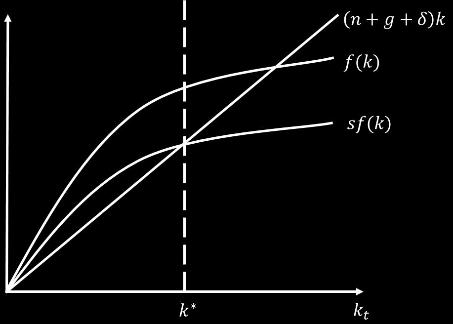
38 Model Dynamics III

39 Model Dynamics IV Taking natural logarithm on k, thus lnk t = lnk t lna t lnl t. Then, we take derivative on both sides, k t K = t g n k t K t = s Y t K t δ g n = s f (k t) k t (n + g + δ)

40 Balanced Growth Path I ˆ The balanced growth path is dened in the economy such that all variables (including aggregate variables, variables in per worker form and variables in per eective worker form) grow at constant rates. ˆ The growth rates could be zero, negative or positive. The growth rates of variables do not have to be the same. Recall the transformation, k t = K t A t L t, taking logarithm on both side, lnk t = lnk t lna t lnl t. And we take derivative on both sides, k t K = t A t L t. k t K t A t L t

41 Balanced Growth Path II By assumption, labor and knowledge are growing at rates n and g, respectively. k t = k on steady state, thus k t = 0. Thus, k t K = t n g. k t K t K t K t = n + g. For the growth rate of Y t, consider k k = s f (k) k (n + g + δ) = s y (n + g + δ) k

42 Balanced Growth Path III At the steady state, we have y = k n+g+δ s, Thus, k t = ẏt Y = t A t L t. k t y t Y t A t L t Y t Y t = n + g. Finally, capital per worker, K/L, and output per worker, Y /L, are growing at rate g. For example, if we dene K i = K t L t represents the capital stock per capita (per person), we have K it K it = g.

43 Balanced Growth Path IV ˆ Note that this growth rate is exogenousthere's nothing in the model that a country can change to increase its long-run growth rate. ˆ The growth rate of output per capita in the steady state does not depend on the savings rate, population growth rate, income level, or amount of capital. ˆ It depends ONLY on the rate of exogenous technological progress.

45 Consumption and Savings I ˆ Since an exogenous fraction s of income is saved, we also know that the fraction (1 s) is consumed each period. In other words, C = (1 s)y, or in terms of eective units of labor, c = (1 s)y. ˆ In the steady state, consumption per worker grows at rate g. (Consumption per eective unit of labor, of course, is constant in the steady state.) ˆ Let's use discrete time here. Following the text, let c denote consumption per eective unit of labor on the balanced growth path (i.e., in the steady state). (Note! It is a steady state in terms of eective units of labor; it is a balanced growth path in per capita terms.) On the balanced growth path, sy = sf (k) = (n + g + δ)k, so c = f (k ) (n + g + δ)k

46 Consumption and Savings II ˆ Recall that k depends on n, g, δ, and s. We are interested in how a (permanent) change in the steady state aects the balanced growth path of consumption: c s = [f (k (s,n,g,δ)) (n + g + δ)] k (s,n,g,δ). (5) s ˆ At the steady state, we have sf (k ) = (n + g + δ)k. Take derivatives on both sides respect to s, we have f (k ) + f (k ) k s = (n + g + δ) k s.

47 Consumption and Savings III k s = = f (k ) (n + g + δ) sf (k ) = k f (k ) (n + g + δ)k sk f (k ) k f (k ) sf (k ) sk f (k ) > 0. Thus, k is positively related to s. Thus, the overall eect of saving rate on consumption depends on whether f (k ) is greater or less than (n + g + δ). In the steady state of this model, income goes only to (1) consumption, and (2) replacing lost capital per eective unit of labor (the fraction (n + g + δ) of k).

48 Consumption and Savings IV ˆ Recall also that we have diminishing returns to capital in this model. That means that f (k) is decreasing in the overall level of k. At low levels of k, then, f (k ) is generally greater than (n + g + δ), so that an increase in the savings rate increases steady-state consumption per ELU. At higher levels of k, though, f (k ) is less than (n + g + δ), so that the increase in savings causes a decrease in steady-state consumption per ELU. ˆ The golden rule level of savings, or the golden rule capital stock: the level of savings that maximizes steady-state consumption per eective labor. ˆ The rst-order conditions imply that consumption is maximized at the point where f (k) = (n + g + δ). This is the point at which the slopes of f (k) and (n + g + δ)k are equal.

49 Consumption and Savings V ˆ Note that this means that, although increasing the savings rate always increases the balanced growth path of income per worker, it does not always increase the balanced growth path of consumption.

50 Consumption and Savings VI

51 Solow Model with a Cobb-Douglass production function I ˆ Let's work through an example with a Cobb-Douglass production function Y t = K α t (A t L t ) 1 α. ˆ The other notation is standard. The intensive form of the production function is then y = F ( K AL,1) = ( K AL) α, so y = k α. We have sk α = (n + g + δ)k, and solve for the steady-state k : k s = ( n + g + δ )1/(1 α) (6)

52 Solow Model with a Cobb-Douglass production function II ˆ This is the steady-state level of capital per eective unit of labor (ELU). It is increasing in s, the savings rate, and decreasing in n (population growth), g (the rate of technological progress), and δ (depreciation). Also note that you could easily substitute this into the production function: y = k α. ˆ Recall the condition of golden rule level of consumption, = n + g + δ, thus we have αk α 1 t s Golden = α. ˆ Recall that s and n have no eect on the long-run growth rate of income per capita they only aect the steady-state level of income (per ELU).

53 Solow Model with a Cobb-Douglass production function III ˆ In the steady state, income per capita does grow, at g. Notice that a higher rate of technological growth (g) means two things: ˆ the economy grows faster in per capita terms in the steady state; ˆ the steady-state level of income (per ELU) is lower. The second is because with a higher g, more investment has to go to maintaining the existing level of capital per worker. ˆ It's more intuitive to think of this in terms of population growth, which is the same idea: the faster is population growth, the more investment needs to go to maintaining the current level per worker for the new workers.

54 Exercise Think about how each of the following developments aects the equilibrium diagram of the Solow model. Evaluate the eect on the steady state value of k: (a) The rate of depreciation falls; (b) the rate of technological progress rises; (c) population growth rate increases; (d) saving rate increases.

56 Human Capital I In order to enrich our model, we want to include human capital. Human capital is a term we use to represent the stock of skills, education, competencies and other productivity-enhancing characteristics embedded in labor. Put dierently, human capital represents the eciency units of labor embedded in raw labor hours. Adding human capital to theory: the production function becomes: Y t = K α t H β t (A t L t ) 1 α β (7) H is the stock of human capital. We assume that it accumulates and depreciates exactly like physical capital; the savings rates for physical and human capital dier and are given by s k and s h respectively. Two rates of depreciation are, δ k and δ h, respectively.

57 H(t) A(t)L(t) Human Capital II Let h(t) =, the laws of motion of these two types of capital goods is given by k t = s k y t (n + g + δ k )k t ḣ t = s h y t (n + g + δ h )h t (8) where y t = k α t h β t. Assuming that α + β < 1, or that there are decreasing returns to all capital. At steady states, k = ḣ = 0. k t = s k kt α 1 h β t (n + g + δ k ) = 0 k t k t = s h kt α h β 1 t (n + g + δ h ) = 0 k t h t k t = s h s k n + g + δ k n + g + δ h

58 Human Capital III Thus, the steady states for the two capital stocks: k = [ ( s k n + g + δ k ) 1 β ( s h n + g + δ h ) β ] 1 1 α β h = [ ( s k n + g + δ k ) α ( s h n + g + δ h ) 1 α ] 1 1 α β If δ k = δ h = δ, we have s1 β k s β h k = ( ) 1/(1 α β) ; n + g + δ k h = ( sα k s1 α h n + g + δ h ) 1/(1 α β) (9)