STATISTICAL MODELING OF LONGITUDINAL SURVEY DATA WITH BINARY OUTCOMES

Transcription

1 STATISTICAL MODELING OF LONGITUDINAL SURVEY DATA WITH BINARY OUTCOMES A Thesis Submitted to the College of Graduate Studies and Research in Partial Fulfillment of the Requirements for the Degree of Doctor of Philosophy In the Canadian Centre for Health and Safety in Agriculture College of Medicine University of Saskatchewan Saskatoon, SK, Canada By SUNITA GHOSH Copyright Sunita Ghosh, December All rights reserved.

2 PERMISSION TO USE In presenting this thesis in partial fulfillment of the requirements for a Postgraduate degree from the University of Saskatchewan, I agree that the Libraries of this University may make it freely available for inspection. I further agree that permission for copying of this thesis in any manner, in whole or in part, for scholarly purposes may be granted by the professor or professors who supervised my thesis work or, in their absence, by the head of the Department or the dean of the College in which my thesis work was done. It is understood that any copying or publication or use of this thesis or parts thereof for financial gain shall not be allowed without my written permission. It is also understood that due recognition shall be given to me and to the University of Saskatchewan in any scholarly use which may be made of any material in my thesis. Requests for permission to copy or to make other use of material in this thesis in whole or part should be addressed to: Director, Canadian Centre for Health and Safety in Agriculture (CCHSA) College of Medicine University of Saskatchewan i

3 ABSTRACT Data obtained from longitudinal surveys using complex multi-stage sampling designs contain cross-sectional dependencies among units caused by inherent hierarchies in the data, and within subject correlation arising due to repeated measurements. The statistical methods used for analyzing such data should account for stratification, clustering and unequal probability of selection as well as within-subject correlations due to repeated measurements. The complex multi-stage design approach has been used in the longitudinal National Population Health Survey (NPHS). This on-going survey collects information on health determinants and outcomes in a sample of the general Canadian population. This dissertation compares the model-based and design-based approaches used to determine the risk factors of asthma prevalence in the Canadian female population of the NPHS (marginal model). Weighted, unweighted and robust statistical methods were used to examine the risk factors of the incidence of asthma (event history analysis) and of recurrent asthma episodes (recurrent survival analysis). Missing data analysis was used to study the bias associated with incomplete data. To determine the risk factors of asthma prevalence, the Generalized Estimating Equations (GEE) approach was used for marginal modeling (model-based approach) followed by Taylor Linearization and bootstrap estimation of standard errors (design-based approach). The incidence of asthma (event history analysis) was estimated using weighted, unweighted and robust methods. Recurrent event history analysis was conducted using Anderson and Gill, Wei, Lin and Weissfeld (WLW) and Prentice, Williams and Peterson (PWP) approaches. To ii

4 assess the presence of bias associated with missing data, the weighted GEE and patternmixture models were used. The prevalence of asthma in the Canadian female population was 6.9% ( ) at the end of Cycle 5. When comparing model-based and design- based approaches for asthma prevalence, design-based method provided unbiased estimates of standard errors. The overall incidence of asthma in this population, excluding those with asthma at baseline, was 10.5/1000/year ( ). For the event history analysis, the robust method provided the most stable estimates and standard errors. For recurrent event history, the WLW method provided stable standard error estimates. Finally, for the missing data approach, the pattern-mixture model produced the most stable standard errors To conclude, design-based approaches should be preferred over model-based approaches for analyzing complex survey data, as the former provides the most unbiased parameter estimates and standard errors. iii

5 ACKNOWLEDGEMENTS I would like to sincerely thank my thesis supervisors Dr. Punam Pahwa and Dr. Donna C. Rennie for their unconditional moral support, inspiration, advice and 'only high-quality work and not less' has inspired me in one and many ways throughout the four years of my PhD and in preparation of my thesis. I owe them gratitude for showing me what real research means. I would also like to thank all my PhD committee members, Dr. Cheryl Waldner, Dr. Bonnie Janzen and Dr. James Dosman for monitoring my work, taking effort in reading my thesis and providing me with valuable comments which have been extremely helpful in completing my thesis work successfully. I sincerely thank Dr. Helen H. McDuffie who was my thesis committee chair for almost three years for her never ending support and her belief in me. Also I would like to sincerely thank Dr. James Dosman for providing me with my own office space and a computer during the training. Special thanks also go to my present committee chair Dr. Niels Koehncke. I would like to sincerely thank Founding Chairs, development fund of the Canadian Centre for Health and Safety in Agriculture and College of Graduate Studies and Research, University of Saskatchewan for providing me financial support during the four year study period. Also would offer my gratitude to Presidents Fund, College of Medicine and Founding Chairs, University of Saskatchewan for providing me financial support to attend national and international conferences. Special thanks goes to the Quebec Inter-university Centre for Social Statistics (QICSS) summer school for providing me with financial support (covering my registration, travel, and iv

6 accommodation cost during my stay in Montreal, Quebec) in attending two special topic courses required for my thesis work and not offered at my host University. I m grateful to the Remote data access unit for providing me remote access to the National Population Health Survey (NPHS) dataset on which my thesis was based. Sincere thanks to Catherine Dick at the remote data access unit for successfully running my programs and returning me with the output. A special thank goes to Dr. J.N.K. Rao who provided me with the idea of using Survey GEE methods which forms an important part of my thesis. Last but not least I would like to thank Dr. Susana Rubin-Bluer and Abdel Nasser Saidi of Statistics Canada for their support with the SAS macro, without their help I couldn t have achieved my thesis objective successfully. v

7 DEDICATION This thesis is dedicated to my husband Moni Shankar Jena and our son Avigna and new addition to our family little Avyukta. Moni s support, love and faith in me have kept me going and helping me to finish my thesis. Avigna and Avyukta were born during my PhD thesis. Their births have provided with me an additional joyful dimension to my life. I m grateful for their love and support which has helped me even in the hardest part of my academic career. vi

8 TABLE OF CONTENTS PERMISSION TO USE... i ABSTRACT... ii ACKNOWLEDGEMENTS...iv DEDICATION...vi TABLE OF CONTENTS... vii LIST OF TABLES...xii LIST OF FIGURES...xv LIST OF ABBREVIATIONS...xvii CHAPTER 1 - INTRODUCTION Rationale Study objectives...6 CHAPTER 2 - LITERATURE REVIEW Introduction Statistical methods for binary outcomes from longitudinal non-survey data Generalized Estimating Equations Marginal models for non-survey data Event history analysis for non-survey data Variance corrected models Frailty models Missing data due to dropouts Cross-sectional and longitudinal Complex Survey designs Analysis of complex survey data Longitudinal complex survey data Marginal models for survey data Even history analysis for survey data Epidemiology of adult asthma International asthma prevalence Adult asthma prevalence in Canada Gender differences...41 vii

9 2.4.4 Rural/ urban differences for asthma Other risk factors of asthma...44 CHAPTER 3 - DATASET DESCRIPTION Study design Sampling strategy Longitudinal sample weights Description of National Population Health Survey Study population Data collection and non-responses Study variables Outcome variable of interest Risk factors of asthma in adult population Data Management...62 CHAPTER 4 - METHODS: MODELS FOR DISCRETE LONGITUDINAL SURVEY DATA Introduction Objective 1: Marginal modeling approach Crude prevalence estimation Rao and Wu Bootstrap Method for variance estimation of crude prevalence Taylor Linearization Method Adjusted prevalence rates using marginal modeling approach GEE for binary data Survey GEE accounting for the design effects Statistical application: Objective Crude prevalence of asthma Adjusted prevalence of asthma using marginal modeling approach Objective 2: proportional hazard model Crude incidence analysis Cox s proportional hazard model Discrete proportional hazard model...82 viii

10 Discrete survival and the complimentary log-log link Statistical application: objective Data arrangement for incidence analysis Crude incidence analysis Adjusted incidence of asthma Objective 3: Variance corrected and frailty models Variance corrected models Andersen and Gill approach Wei, Lin and Wiessfeld (WLW) model Prentice, William and Peterson (PWP) model Frailty Model Approach Gamma frailty Statistical application: objective Arrangement of the data for recurrent survival data Computer software of Variance corrected and frailty model Objective 4: Missing data analysis Notation and arrangement of the data Weighted Generalized Estimating Equation (WGEE) Random effects models Statistical application: objective Data arrangement for handling missing data Application of WGEE analysis Application of Random Effect Modeling CHAPTER 5 - RESULTS: MODELS FOR DISCRETE LONGITUDINAL SURVEY DATA Introduction Subjects Descriptive analysis Objective 1: Prevalence estimation Crude prevalence rate calculation Marginal modeling approach for cross-sectional survey data ix

11 5.4.3 Marginal modeling approach for the longitudinal survey data Computation of parameter estimates Interpretation of results Interpretation of the main effects odds ratios Interpretation of interaction terms Predicted probability calculated for the significant effect modifiers Objective 2: Incidence analysis Crude incidence rate calculation Incidence density rate Crude rate ratio using STMH command Proportional hazard regression models Objective 3: Variance corrected and frailty models Fitting variance corrected models Interpretation of the WLW model Objective 4: Missing data analysis Marginal models Random Effect Models Conclusion CHAPTER 6 - DISCUSSION Introduction Objective 1: To compare the design-based and model-based methods for the marginal modeling approach Objective 2: To compare the design-based and model-based methods for event history data Objective 3: To compare the variance corrected and frailty models for recurrent survival data using both the design-based and model-based approach Objective 4: To compare the robustness of data for completers versus incompleters using missing data analysis Prevalence and incidence estimation of asthma in the adult Canadian female population Limitations and advantages of using the NPHS data x

12 6.8 Conclusion and future studies BIBILIOGRAPHY APPENDIX A A.1 Notation of matrices and vector A. 2 Glossary of statistical terms used for survival analysis APPENDIX B B. 1 Guidelines of Statistics Canada for result publication B.2 NPHS selected questionnaires Appendix C C.1 SAS Macro: Survey GEE C.2 SAS macro for Bootstrap analysis C.3 SAS macro for WGEE analysis APPENDIX D D. 1 Remote access to National Population Health Survey data APPENDIX E E. 1 Exemption from ethics approval letter xi

13 LIST OF TABLES Table 2.1 Major Canadian studies of asthma prevalence in the general adult population...39 Table 2.2 International prevalence of doctor diagnosed asthma among males and females...42 Table 3.1 Longitudinal sample size of Cycle1 and Cycle 5 by Province...53 Table 3.2 Response, refusal, attrition and cumulative attrition rate of 17,276 panel members for each Cycle...57 Table 3.3 Income adequacy level based on the household income and size...62 Table 4.1 Recurrent asthma events included in the analysis to fit parsimonious model of asthma free females at the end of Cycle Table 4.2 Possible missing data patterns and the frequency of the outcome variable Self reported health professional diagnosed asthma Table 5.1 Number of participants (%) stratified by asthma status for each Cycle of participation Table 5.2 Baseline characteristics of the covariates included in the analysis, n (%) Table 5.3 Number of participants (%) stratified by cycles and province Table 5.4 Asthma prevalence and 95% confidence interval of adult females in years age group Table 5.5 Asthma prevalence and 95% CI of females for the age group years stratified by location (Rural/Urban) Table 5.6 Asthma prevalence (95% confidence interval) for all the important covariates included in the final model xii

14 Table 5.7 Comparison of design-based versus model-based, adjusted odds ratio (95% confidence interval) for Cycle 1 ( ) Table 5.8 Estimates (Standard Errors) and Odds Ratio (95% Confidence Interval) with Exchangeable correlation matrix Table 5.9 New asthma cases stratified by Cycles Table 5.10 Weighted and unweighted analysis of Incidence density rates (per 1000 person years) of asthma stratified by Cycle and each categorical covariate Table 5.11 Crude stratified rate ratio of asthma incidence for covariates/risk factor using the STMH command in STATA Table 5.12 Methods and the STATA command used to achieve objective Table 5.13 Discrete and Cox s proportional hazard model (Robust standard error), unadjusted hazard ratio of covariates/risk factors Table 5.14 Model-based Discrete and Cox s proportional hazard model; unadjusted hazard ratio of covariates/risk factors Table 5.15 Discrete and Cox s proportional hazard model (Robust standard error), adjusted hazard ratio of covariates/risk factors Table 5.16 Model-based adjusted hazard ratio Discrete and Cox s proportional hazard model of covariates/risk factors Table 5.17 Distribution of first and subsequent episodes of asthma and censoring during the follow-up time Table 5.18 Weighted and unweighted hazard ratio (HR) and 95% confidence interval using Anderson Gill (AG) approach xiii

15 Table 5.19 Weighted and unweighted hazard ratio (HR) and 95% confidence interval using Wei, Lin and Weissfeld (WLW) approach Table 5.20 Weighted and unweighted hazard ratio (HR) and 95% confidence interval using gap time/total time Prentice, William and Peterson (PWP) approach Table 5.21 Parameter estimates (standard errors) and odds ratio (95% confidence interval) for GEE with survey weights and weighted generalized estimating equation (WGEE) Table 5.22 Parameter estimates (standard errors) for a generalized linear mixed model (GLMM) assuming Penalized Quasi Likelihood (PQL) restricted maximum likelihood and maximum likelihood approach with and without drop variable in the model Table 5.23 Summarizing the final model selected for interpretation xiv

16 LIST OF FIGURES Figure 3.1 Complex Survey Design for Longitudinal Health Survey data...49 Figure 3.2 Flowchart showing selection of the final sample size...55 Figure 4.1 Statistical methods available for longitudinal data assuming simple random sampling and complex survey sampling...65 Figure 4.2 Methods used to obtain prevalence of asthma...78 Figure 4.3 Diagrammatic representation of selecting new cases of asthma at each cycle...88 Figure 4.4 Methods used to calculate incidence of asthma...93 Figure 4.5 Variance corrected methods used for recurrent event data Figure 4.6 Missing data patterns: using an example with three time point study Figure 4.7 Coding scheme of missing data pattern, shown with the help of an example with three time points (O-observed; M-missing) Figure 4.8 Missing data analysis using marginal and random effect modeling Figure 5.1 Asthma cases in the study sample of female participants in the age group years stratified by Cycle of participation Figure 5.2 Mean predicted probability of asthma stratified by location ( = rural; = urban) Figure 5.3 Mean predicted probability of asthma stratified by exposure to second hand smoke (---- = exposure to second hand smoke; = no exposure to second hand smoke) Figure 5.4 Mean predicted probability of asthma stratified by rural/urban location and smoking status ( = rural; = urban) xv

17 Figure 5.5 Mean predicted probability of asthma stratified by rural/urban location and socio-economic status ( = rural; ---- = urban) Figure 5.6 Mean predicted probability of asthma stratified by ethnicity (Caucasian/non- Caucasian) and socio-economic status ( = Caucasian; ----=non-caucasian) Figure 5.7 Mean predicted probability of asthma stratified by smoking status and age groups (-- -- = years; = years; = years; = years) Figure 5.8 Mean predicted probability of asthma stratified by socio-economic status and age group (-- -- = high income; = middle income; = low income)..155 Figure 5.9 Frequency distribution of asthma recurrence in females from Cycle 2 to Cycle xvi

18 LIST OF ABBREVIATIONS AFT AG BHR BMI BRFSS BRR CC COPD EB ECRHS EM ESS GEE GINA GLM GLMM GT-UR IID IUTALD LOCF LWA Accelerated failure time Anderson and Gill Model Bronchial hyper responsiveness Body mass index Behavioral Risk Factor Surveillance System Balanced repeated replication Complete case analysis Chronic Obstructive Pulmonary Disease Empirical Bayes European Community Respiratory Health Survey Expectation-maximization Enquete sociale et de Sante Generalized Estimating Equation Global Initiative for Asthma Generalized Linear Models Generalized linear mixed model Gap time- unrestricted Identically Independently Distributed International Union Against Tuberculosis and Lung Disease Last observation carried forward Lee, Wei and Amato xvii

19 MAR MCAR MI ML MNAR MQL NPHS PPS PQL PSU PWP REML SRS TT-R WGEE WLW Missing at random Missing completely at random Multiple imputation Maximum likelihood Missingness not at random Marginalized Quasi Likelihood National Population Health Survey Probability proportional to size Penalized Quasi Likelihood Primary Sampling Units Prentice, William and Peterson Restricted maximum likelihood Simple random sample Total Time Restricted Weighted generalized estimating equations Wei, Lin and Weissfeld xviii

20 CHAPTER 1 - INTRODUCTION 1.1 Rationale Large national health surveys are an invaluable source of information on the incidence and prevalence of disease and associated risk factors. Such surveys require the use of multi-stage sampling designs to collect information. Multi-stage sampling procedures involve a number of steps including stratification, clustering, random sampling of households within clusters with unequal inclusion probabilities, and selecting individuals within responding households. Hence, the three features of multistage design are: stratification, clustering and unequal inclusion probabilities. To obtain consistent estimates of parameters and their variances, the analysis of survey data should account for the sampling design. The first feature of multi-stage sampling, stratification, is achieved by creating homogeneous subgroups or strata. These homogeneous subgroups created by stratifying the probability samples assist in minimizing sampling error [4], reducing the variance of parameter estimates, and making the population subgroups more adequately representative of the overall population [5]. Stratification also aids in increasing statistical efficiency [4]. 1

21 The second feature of multi-stage design is clustering. Compared to data collected using a simple random sampling approach, data collected by a multi-stage design incorporating a clustering effect produces more stable parameter estimates [5]. However, due to a clustering effect, the multi-stage method of data collection results in larger standard errors and variances. [5] Hence, clustering underestimates the true population variance and results in loss of statistical efficiency [5]. The third feature, weighting, accounts for unequal inclusion probabilities and non-response. The sampling weights assists in reducing bias in the parameter estimates, and can result in large standard errors if the variance of the weights is large [4]. Statistical methods for cross-sectional survey designs are well developed and can be easily applied through commercial software such as SAS 1, SUDAAN 2, STATA 3 and WESVAR 4. The software can handle the complexities of both design-based and model-based statistical approaches used with data from cross-sectional surveys. Contrary to the analysis of data from cross-sectional survey designs, the analysis of data from longitudinal survey designs can be more complicated. The analysis of longitudinal survey data should not only account for stratification, clustering and an unequal inclusion probability, but must also take into account the within-subject correlation arising from repeated observations or missing data on the same individual over time. Ignoring the sampling design may result in severely biased estimates, leading to false inferences, especially when the outcome variable is correlated with design variables not included in the model [6]. 1 SAS Institute, Inc. Cary, NC, version ( 2 SUDAAN, Research Triangle Institute, 2005 ( 3 STATA, Stata Corp LP, ( 4 WESVAR, Westat Inc., 2006 ( 2

22 There is limited work conducted with complex survey data sets that are longitudinal in nature and with binary outcomes. Some recent work in the area of longitudinal survey data analysis has been conducted by Skinner and Holmes [7] and Feder et al. [6], who have used the random effects modeling approach for continuous outcomes. Rao [3] proposed the use of a marginal modeling approach with binary outcomes, while Lawless [8] proposed the use of event history analysis for binary outcomes. These methods focused on design-based approaches. Model-based methods have also been used and have been compared to design-based methods for crosssectional survey data [9], but their use is limited with longitudinal survey data. There is ongoing debate as to which of these approaches is best for the analysis of survey data [10]. Results from complex survey analyses that have used the appropriate statistical methods can be generalized to the specific target population of interest. In this thesis, the National Population Health Survey (NPHS), a multi-stage complex longitudinal survey dataset, was used. The primary purpose of this study was to examine the prevalence and incidence of asthma and associated risk factors among adult women using different statistical approaches, ultimately evaluating the statistical efficiency of these different approaches. Asthma is a chronic respiratory disease and its symptoms include wheezing, shortness of breath, tightness of chest and coughing [11]. Research conducted in Canada and other countries has shown that asthma prevalence among the adult population is rising and is more predominant in western and developed countries [12]. During adulthood, asthma prevalence appears to decrease with age, however, there is a change in the gender distribution of asthma from childhood to adulthood with more 3

23 [12] females affected than males during adulthood [11]. These finding are supported by several studies of adult populations which clearly show the higher prevalence and incidence of asthma among females compared to males [13-19]. Research has focused on rural/urban differences in the prevalence and incidence of asthma among adults [20-22]. While researchers have reported results adjusted for gender, they have not specifically examined the role of gender by location. In Canada, cross-sectional studies of asthma prevalence show that between 1994 and 2003, the overall prevalence of asthma among persons aged 12 years and over increased and then plateaus. Asthma prevalence is consistently higher among females than males, indicating that the increase in overall prevalence of asthma is primarily due to an increase in prevalence among females. To date, most of the research on the prevalence and incidence of asthma in adult populations has focused on gender differences [13, 15, 17, 18]. Further research is needed using longitudinal study designs to explore the reasons behind the higher prevalence and incidence of asthma among the female population in Canada. Beginning in 1994, the NPHS longitudinal survey has collected health and other information of the Canadian population every two years using a multi-stage sampling design 5. This dataset is unique in that the results obtained can be generalized to the Canadian population. To date, the NPHS dataset has not been analyzed longitudinally using all five cycles for a comparative study of model-based and design-based approaches. As well, the dataset has not been used to study the prevalence and incidence of asthma and associated risk factors using appropriate statistical technique to account for the complex survey design. 5 Refer to Chapter 4 for a detailed description of the NPHS data set 4

24 This thesis compares the design-based and model-based methods for longitudinal survey data with a binary asthma outcome. Although these methods have been discussed separately in literature, there has been no comparison between them using the NPHS dataset with asthma as the outcome. The uniqueness of the thesis is that it compares the model-based and design-based approaches for marginal modeling, survival analysis techniques, and variance corrected estimation methods for recurrent events. In addition, this thesis explores the effectiveness of various statistical methods for handling missing data commonly occurring in longitudinal surveys. 5

25 1.2. Study objectives The objectives of the present thesis are the following: 1. To compare the design-based and model-based methods for the marginal modeling approach a. To determine the prevalence of asthma and associated risk factors in the adult Canadian female population, taking into account the complexity of the multi-stage sampling process. 2. To compare the design-based and model-based methods for event history data. a. To determine the incidence of asthma and associated risk factors in the adult Canadian female population. 3. To compare the variance corrected and frailty models for recurrent survival data using both the design-based and model-based approach. 4. To compare the robustness of data for completers versus incompleters using missing data analysis. 6

26 CHAPTER 2 - LITERATURE REVIEW 2.1 Introduction Statistical methods used for analyzing data obtained from standard longitudinal studies can be easily extended to analyze longitudinal survey data. The major difference between standard longitudinal studies and longitudinal complex surveys is the sampling design. Simple random sampling (SRS) designs are often used to collect data for standard longitudinal studies. Commonly, for longitudinal complex surveys, stratified multi-stage sampling designs are used. Other types of sampling designs (e.g. stratified sampling, systematic sampling, cluster sampling etc.) are also available for complex surveys. In large-scale national surveys, multi-stage designs are used because of economical reasons. Such designs substantially reduce the traveling cost of interviewers. However, multi-stage sampling techniques have drawbacks too. Clusters tend to be internally homogenous and this increases the standard errors of estimates, which in turn, decreases the statistical efficiency. Another disadvantage arising due to clustering is that in such sampling, the variation arises due to between-cluster variation and within-cluster variation. Analysis of survey data should be able to account for the additional source of variation. The variation within clusters contributes to the total variation. The problem arising due to clustering can be easily rectified at the design 7

27 stage, by using a large number of strata and then drawing more than one cluster per strata. For example, in the NPHS, approximately 3 clusters per strata are chosen. The statistical methods discussed in the following sections are divided into longitudinal non-survey data and longitudinal survey data. The methods for longitudinal non-survey data analysis are reviewed first because these methods are extended to analyze longitudinal survey data. Statistical methods for survey data analysis must consider the design effects to achieve unbiased and correct estimates and their standard errors. Analytical or resampling techniques are then used to obtain variance estimates. 2.2 Statistical methods for binary outcomes from longitudinal non-survey data Research in longitudinal data analysis was first started by Wishart [23], and gained momentum in developing models for linear outcomes around 1950 s with the availability of computing facilities for statistical purposes [24]. The early efforts made by Box [25], Geisser and Greenhouse [26], Potthoff and Roy [27], Rao [28, 29] and Grizzle and Allen [30] have resulted in the rich variety of models for Gaussian data [24]. However, for non-linear outcomes such as binary outcomes, few methods were available until One of the main reasons for the inadequate development of analytical methods for non-linear outcomes with longitudinal data was the lack of multivariate distribution. For non-gaussian longitudinal data, additional information is required to determine the likelihood, as the first two moments are not enough to determine the likelihood function. The mean and the variance could not be separated in non-gaussian data, as the mean and variance is related and estimated using a single parameter [31] as in binomial distribution variance is a function of mean (µ*(1-µ)) and 8

28 for Poisson distribution variance is equal to the mean (µ). The impossibility of modeling the mean and variance separately results in interpretational and computational problem in non-gaussian data [24]. An alternative approach, which has gained a lot of attention, is the introduction of Generalized Linear Model (GLM) by Nelder and Wedderburn [32]. GLM extends the ordinary regression models to include the non- Gaussian responses such as discrete outcomes, and special cases of Poisson and survival. In a way, GLM unifies the different regression models [33]. GLM has three components: (i) a random component which identifies the response variable and its probability distribution; (ii) a systematic component which identifies the explanatory variables used in the linear predictor function; and (iii) a link function that relates the random and the systematic components [34]. GLM is a linear model that has a distribution in natural exponential family. The traditional maximum likelihood approaches cannot be used for non- Gaussian data as the integral does not have a closed form, unlike the Gaussian data [35]. Numerical integration techniques are required to evaluate the likelihood. The likelihood estimates are often intractable and involves solving other nuisance parameters besides estimating regression coefficients, even with these additional assumptions [35]. To overcome these problems, Liang and Zeger [1] introduced the Generalized Estimating Equation (GEE). The GEE method is based on multivariate quasi likelihood theory and it can handle the complexities of longitudinal data. 9

29 2.2.1 Generalized Estimating Equations The GEE approach proposed by Liang and Zeger [1] is a class of estimating equations which take into account the correlation arising due to a longitudinal study design, resulting in increased efficiency of standard error estimates. introduced by Wedderburn [36], the GEE approach is based on quasi likelihood theory and can be used for continuous as well as for discrete outcome [1, 37]. The GEE method is a multivariate generalization of quasi-likelihood, and this method is mainly proposed for marginal modeling with GLM [1]. This method avoids the use of multivariate distribution by assuming a functional form for marginal distribution at each time, making it useful for non-gaussian outcomes [1]. The advantage of using the GEE method is that the solutions are consistent, i.e. the estimate of β are nearly efficient and asymptotically Gaussian, even when the time dependence is misspecified [37, 38]. Considering the GEE approach, let Y i = (y i1,...y ini ) T denotes the outcome vector for subject (i=1,.n); µ i = (µ i1,.., µ ini ) T denotes the mean vector, where µ it = E(Y it ); and X i = (x i1,..,x ini ) T be a n i x p matrix of explanatory variables for subject i. The GEE approach also assumes a working correlation matrix R(α) for Y it depending on parameter α. Let R(α) be the n x n symmetric matrix and α be an s x 1 vector, then R(α) as defined by Liang and Zeger [1] is V i =A 1/2 i R(α)A 1/2 i /φ And v i = cov (Y i ) if R is true correlation matrix for Y i, and A i = diag {a (θ it )} When we have univariate GLM, then the quasi likelihood estimating equation have the form 10

30 i µ β T [ y )] = 0 1 = v( µ ) i(β i i i µ (2.2.1) The analog of this in multivariate is the generalized estimating equation given by Liang and Zeger [1] N i= 1 D [ ( β )] = 0 T T i Vi i µ i T { a (θ)} where i y (2.2.2) D i = = A i i X β ( µ i / β) is a n i x p matrix i A i denotes a diagonal matrix with main diagonal elements a i (θ it ) i is a diagonal matrix with elements θ it / η it a n x n matrix. It was shown by Liang and Zeger [1] that as the number of clusters n increases, asymptotic normality and consistency was obtained. β β N 0, V ) and V G = lim V G,n with n 1 1 ( G (2.2.3) n n n V G = lim T 1 T 1 1 T 1 n n DV i i Di DV i i COV( Yi) Vi Di DV i i D (2.2.4) i i= 1 i= 1 i= 1 When COV(Y i )=V i, and the working correlation structure is true one, then the asymptomatic covariance matrix V G simplified to n T 1 DV i i D i i= 1 1 The β estimated using the GEE approach is efficient and consistent even if the covariance structure of Y it is incorrectly specified [1]. However, the correlation structure in case of discrete data is not one of the best ways to express the withinsubject correlation [34]. An alternative approach is the use of odds ratios, by modeling 11

31 the log odds ratio for pairs in a cluster as exchangeable [34, 39, 40]. Another alternative is the iterative alternating logistic regression algorithm proposed by Carey [41]. Longitudinal data analysis has three extensions of the generalized linear models, (GLM) namely marginal models, random effects models and transitional models. In linear models with continuous outcomes, the interpretation of the regression parameter is independent of the correlation structure. However for non-linear models, different assumptions of correlation structure will result in regression coefficients with distinct interpretations [35]. The regression coefficient for linear models can have a marginal interpretation for all three approaches but this is not true for non-linear data [35]. Zeger et al. [42] showed that for the logistic model, the β estimate of marginal and random effects models are not equal, but β 2 2 1/2 * ( cv + 1) β (2.2.5) where c is a constant and is equal to 16 3 /(15 π ) with c2=0.346, and 2 v is the variance. β is estimated using a marginal model and β* is estimated using a random effects model. However, it is only in limited cases that the relationship between transitional and marginal models can be established for non-linear models [35]. As a consequence, one should be careful in the choice of the model for non-linear outcomes and this choice should depend on the research question being addressed [35]. discussed. In the next section, the marginal models for non-gaussian outcomes are 12

32 Marginal models for non-survey data In marginal models, the parameters characterize the marginal probability of success at a given point in time when the response is binary [43]. A fully specified marginal model taking into account the correlation and implementing likelihood inference for discrete data, was first proposed by Bahadur [44]. This model was also studied by Cox [45], Kupper and Haseman [46] and Altham [47]. The existence of severe constraints on correlation parameter space was the major drawback of the model proposed by Bahadur [44]. The log-linear models proposed by Bishop et al. [48] were the most widely used probability models for multivariate binary data. The canonical parameters were undesirable and their interpretation was dependent on the number of responses (N). The latter was a major drawback of the model proposed by Bishop et al. [48], because in longitudinal studies, the number of responses can vary across subjects. Diggle et al. [35] tried to build a log-linear model by starting with marginal parameters µ j = Pr (Y j =1), j=1,..n. They proposed a saturated log linear model that had 2 n -1 parameters, which could be obtained in three different ways: (1) using µ j, second and higher order canonical parameters, as proposed by Fitzmaurice et al. [38]. (2) Using log linear models which uses marginal means, as proposed by Bahadur [44] (3) Parameterization of likelihood in terms of marginal odds ratio. The problem with all three models was the unavailability of simple methods to calculate the third and higher order moments, and even with the model fully specified, the likelihood estimates were very complicated [35]. 13

33 To overcome these problems, the GEE approach was proposed by Liang and Zeger [1]. The GEE approach was originally specified for modeling univariate marginal distributions, such as binomial and Poisson [34]. Prentice [49] extended the GEE approach by allowing the simultaneous estimation of parameter vector and variance-covariance matrix. The variance-covariance matrix obtained by these equations was more stable compared to the variance-covariance estimator proposed by Liang and Zeger [9]. Second order GEE were proposed by Zhao and Prentice [50] for continuous or categorical data and by Liang et al. [51] for categorical data. Liang et al. [51] compared the log linear models with the marginal models and suggested that the marginal models can be used when the log linear models become inefficient. Liang et al. [51] referred to the GEE approach proposed by Liang and Zeger [1] as GEE1 and their method as GEE2. The authors showed that the GEE1 method proposed by Liang and Zeger [1] was highly efficient in determining the β estimate, but highly inefficient for estimating α. The GEE2 method was highly efficient in estimating both parameters β, and α. The authors suggest the use of GEE1 when α is a nuisance parameter. Besides this aforementioned point, valid standard errors for βˆ can be obtained using the empirical or sandwich estimator for the cov(β) estimate [1, 37]. An alternative approach to the GEE was given by Carey et al. [41], the so called alternating logistic regression (ALR) method. This method is different from all of the GEE methods discussed above, but because it is based on the odds ratio, has common features of GEE and GEE2 [43]. The advantage of the ALR method [52] is that it requires no working assumption of third and fourth order odds ratios, and combines 14

34 marginal as well as a conditional specification [43]. Work by Zhao et al.[50], Fitzmaurice and Laird [38] and Fitzmaurice et al. [39] made the connection between the GEE approach and the likelihood-based methods [53]. The GEE approach and the sandwich estimator of cov(β) are the most widely used methods in marginal models with discrete outcomes, and most of the available software that implements the use of the GEE approach has made it a very popular technique for models with discrete outcomes [53] Event history analysis for non-survey data Survival analysis is a branch of statistics which primarily deals with death in biological organisms and failure in mechanical systems. Death or failure is called an "event" in the survival analysis literature, and therefore, models of death or failure are generically termed time-to-event models. Research in the field of survival analysis is very much influenced by the regression model developed by Cox [54], introduced in 1972 [45]. Cox extended the Kaplan and Meier [55] life table analyses to include the regression equation. Since then, this technique has become widely used for survival and other censored outcomes. Cox s proportional hazard model for the i th person, given the covariate value x, can be specified by the following equation: ( ) = ( ) λ t x λ t exp( x ( t) β ) (2.2.6) i 0 i where ' β = ( β,..., β p ), is p x 1 column vector of coefficients and λ o (t) represents 1 baseline hazard and is a non negative function of time. 15

35 Assuming no ties, the inference on β can be estimated from the likelihood function: L( β ) δ i n ' exp( β x ) i = ' exp( ) i= 1 j j R ( ) t i β x (2.2.7) where R(t i ) = (j: t j t i ) and (1-δ i ) is an indicator of censoring, and later on Cox derived the equation as partial likelihood function. Survival analysis techniques are also applied to recurring or repeated events, commonly referred to as event history analysis. Examples of repeated events would be recurrent asthma attacks, the occurrence of diabetic retinopathy over time, and the decline of the CD4 count over a small period in AIDS patients. The recurrent events or the repeated event models are correlated, and hence, the assumption of independence is violated. Thus, the major disadvantage of using Cox s model for event history analysis or recurrent failure times data is that the basic assumption of independence is violated. The use of standard analytical approaches for correlated survival data results in reduced efficiency [56] and incorrect estimates of standard errors. Various methods have been developed to account for dependencies due to repeated events at the variance estimation stage. Such methods are called variance corrected and frailty models, and are discussed in the next section Variance corrected models Variance corrected models use robust variance estimation methods to account for heterogeneity among individuals and event dependence [57]. The most commonly used models for multiple events are Anderson Gill (AG), Wei, Lin and Weissfeld 16

36 (WLW) and Prentice, William and Peterson (PWP). The AG model is based on independent increment models, the WLW on marginal models and the PWP on conditional models. Anderson and Gill extended Cox s Proportional Hazard Model to recurrent event data, commonly known as the AG model (also referred to as the independent increment model) [58]. Their generalization was based on the work of the multivariate counting process of Aalen [59]. The AG model intensity process for i th subject is ( ) = ( ) λ t x λ t exp( x ( t) β) (2.2.8) i 0 i and is identical to the Cox model (eq 2.2.7). The AG model is very similar to the Cox s model with a difference in the definition of λ i (t). In the Cox s model λ i (t) equals zero in case of an event whereas for AG model λ i (t) equals 1 as event occurs [60]. Each subject in AG model is treated as a multi-event counting process with independent increments (see appendix A). This model requires a strong assumption of independent increments, especially if ordering of the event is necessary. Another assumption of the AG model is that multiple events for any particular observation are assumed to be independent [61]. The AG model can handle recurrence event data and the model usually assumes that the recurrences follow a non-homogeneous Poisson process and are not affected by the occurrence of earlier events [62]. Wei and Glidden [62] suggest that such strong assumptions can be relaxed by the including time dependent covariates in the model. Wei, Lin and Weisfeld [63] (WLW) modeled the marginal distribution of failure time variable with a Cox s proportional hazards model. This method was based on a semi-parametric approach, with the regression model for the marginal relative risk 17

37 being the parametric component and the marginal baseline hazard and dependence structure constituting the non-parametric part [64]. The usefulness of the semiparametric approach over the full parametric approach was that it did not require as strong assumptions. As well, the modeling of multivariate failure time data has been made possible with the help of computer programs. The hazard function for the j th event for i th subject is ( ) = ( ) λ t x λ t exp( x ( t) β ) (2.2.9) ij j0 i j Here β j represents separate hazard for each event and for strata by covariate interactions [60]. The Conditional Model, or the Prentice, William and Peterson (PWP) model [65] is based on the conditional method and can be analyzed using the partial likelihood principle. The model can be used to model multivariate failure time data. In the PWP model, a second event cannot occur unless the first event has occurred. The time dependent strata vary from event to event. The hazard function is defined as ( ) = ( ) λ t x λ t exp( x ( t) β ) (2.2.10) ij j0 i This equation is similar to the WLW model, the only difference being that λ ij (t) has the value zero until the previous event has occurred. Other marginal models for variance corrected models have been proposed. Wei, Ying and Lin [66] proposed an alternative inference procedure to estimate the variance. This alternative inference approach aids computation of the variances and it does not use the unstable non-parametric approaches. Lee, Wei and Ying [67] proposed a simple linear regression method to analyze highly stratified observations, based on a population averaged model, also known as a marginal model. This method does not require a 18

38 complicated model and the estimates are stable and are not based on non-parametric approaches. These population-averaged models provide valid inferences about the parameter estimates without any distributional assumption. Lee, Wei and Amato [68] used the Cox regression model to model the hazard function of each failure time without imposing dependence among the related failure time observations. Liang, Self and Chang [64] (LSC) also used the marginal distribution approach to make inferences on the parameters in marginal hazard (when there is dependence between individuals). The proposed LSC method used semi- parametric approaches but was different from the WLW marginal model. In LSC model, the relative risk is the parametric component, and the marginal baseline hazard and dependence structure is the non-parametric component. LSC model assumed the dependence structure to be completely unspecified. An alternative method to the Cox model is the accelerated failure time (AFT) model. The AFT model, which is based on regressing the logarithm of survival time over the covariate, can be easily extended to the multivariate case [66, 69]. One of the limitations of variance corrected models is that they are not suitable for modeling competing risks. Further research is needed in this area. Gao and Zhou [70] compared the WLW and LSC models and found that under some regularity conditions (two pairs of observations from different clusters are independent), the LSC method provided robust estimates. However, they suggested the use of the WLW over the LSC method when all covariates are identical for failure data. Guo and Lin (1994) developed a grouped time version of marginal models, which is an advancement of the WLW model. Therneau and Hamilton [71] compared four models 19

39 (AG, WLW, PWP and the Prentice and Cai method) for survival analysis with multiple events per subject. They compared the AG [58] model, the WLW method [63], the PWP [65] and the Prentice and Cai method [72]. The PWP method used the conditional method and Prentice and Cai s method modeled correlations directly using Cox s framework. Therneau and Hamilton [71] suggest the use of AG and WLW because of the availability of computer software to analyze repeated/correlated events data using these approaches. The PWP method is based on the conditional method and can be analyzed using the partial likelihood principle. Both the AG and the PWP models are sensitive to misspecification of dependence structures among recurrence times [63]. The AG, PWP and WLW methods can be analyzed using PROC PHREG in SAS [73]. Wei and Glidden (1997) suggest the use of the models WLW, Wei, Ying and Lin [66], Lee, Wei and Amato [68] and the model by Lee, Wei and Ying [67], as these models are robust and well developed. Kelly and Lim [73] proposed four key elements to characterize the Cox based models: risk interval, baseline hazard, risk set and correlation adjustment. Based on these four key elements, they compared five models: the AG [58], the WLW [63], the PWP-CP [65], the PWP-GT [65] and the LWA [67]. The PWP-GT (gap time) and the PWP-CP (total time) were developed by Prentice, William and Peterson [65]. Gap time is the time from the prior event. Once the event has occurred, the clock restarts. The total time is the time from the start of the treatment. The counting process is similar to total time, except that a subject may have a delayed/censored period before the subject becomes at or a risk for the event. The PWP-CP model is the stratified AG model, 20

40 where the event specific baseline hazard is restricted. Gap time- unrestricted (GT-UR) assumes that the baseline hazard or the risk set is unrestricted and TT-R (Total Time - Restricted) assumes that the baseline hazard or the risk set is restricted or eventspecific. Kelly and Lim [73] concluded from their study that the PWP-GT model and the Total time-restricted (TT-R) model introduced by them are useful for analyzing recurrent data. They suggest the use of PWP-GT when within subject events are independent. The four models compared by Kelly and Lim [73] did not account for the within-subject correlation, even with robust variance. Kelly and Lim [73] recommend the use of PWP-GT and TT-R when within-subject event are independent for analyzing recurrent event data. AG and GT-UR both assume that they have common baseline hazards, but these models cannot be used, as they do not have versatility of event specific model. WLW models are more suitable for multi-type event data, where the baseline hazard is different for each type of events. For example, tumours at different sites of the body [73]. LWA is useful for clustered data when the baseline hazard is the same. For example in clustered data on a pair of eyes [73]. When the WLW model is applied to recurrent data, it leads to an over-estimation of the treatment effect. The LWA model allows the subjects to be at risk several times for same event Frailty models The frailty or random effects model treats the repeated events as a special case of more general unit-level heterogeneity. The random effect is across individuals and constant over time. In Frailty models, a random effect is a continuous variable, which 21

41 describes excess risk or frailty for distinct categories, such as individuals or families. This excess risk or frailty for distinct categories, like individuals and families, is described using a random effect, which is a continuous variable. Computation of frailty is observed as the unobserved covariate [60]. Univariate frailty models were first introduced by Vaupel [74]. Clayton [75] extended the Cox proportional hazard model [45] to multivariate life tables. The model proposed by Vaupel et al. had a fully parametric approach and later Clayton and Cuzick [76] extended the univariate model developed by Vaupel [74]. Their model was a generalization of the proportional hazard model and contained a random effect term to represent heterogeneity of frailty. The model used a non-parametric approach and parameters were estimated by the maximum likelihood method. The proportional hazard model for subject i can be written as λ i (t) = λ o (t) exp(x i β + Z i ω) (2.2.11) where X i and Z i are i th row of covariate matrices X and Z, X and β corresponds to p fixed effects in the model and ω corresponds to a vector which contains information on q unknown random effects or frailties, Z is the design matrix [77]. Huster, Brookmeyer and Self [56] extended the fully parametric model of Clayton [75] and Oakes [78] to include covariate information, and the parameter estimates and robust variance estimators were obtained. Their independent working model (IWM) was computationally simple, but the only limitation was that it ignored the between pair association and resulted in a severe loss of information. On the other hand, the model proposed by Clayton and Oakes took into account between pair associations, but it was computationally intense and associations could only be positive. 22

42 Ross and Moore [79] developed methods for modeling discrete or grouped time survival time when groups or clusters are correlated. They specified the marginal hazard of failure for individual items within a cluster or group by using the linear log odds survival model, and the dependence structure was based on the gamma frailty model [75]. To estimate the parameters, they used a method which combined the GEE method and a pseudo likelihood method. The developed model could handle cluster sizes greater than two and assumed that dependence varied with cluster level covariates. Cox s frailty model [74, 75] allowed between cluster heterogeneity. The mixed effects model developed by Ratcliffe et al. [80] extended the Cox frailty model for repeated measures to include both subject and cluster level random effects. This model was more efficient and less biased, and evaluated the effect of the treatment variable while accounting for the relationship between them. The mixed effects model can be extended to multiple common frailties, and the correlation between cluster level random effects and frailty can be easily overcome by the addition of frailty not linked with random effects. However, this method can be computationally intense. Frailty models or random effects models can also be used when there is correlation present at different hierarchical levels. This multilevel random-effects model for survival data is new, and is gaining momentum due to its application in data where clustering is present between and within subjects at different levels of association. Some of the earlier work in this area is by Rodriguez [81] and Bandeen- Roche [82]. The model proposed by Bandeen-Roche and Liang [82] had the same properties of the multivariate frailty model. Their proposed model took into 23

43 consideration clustering present at multiple levels and reduces to a univariate frailty model in the case of single clustering. A nested frailty model for survival data was proposed by Sastry [83] when there was clustering at two hierarchical levels (community-level and family-level). The parameter estimates were obtained by using the EM-algorithm. Sastry suggests the use of such a model when there is clustering present at different levels as ignoring the clustering will result in upward bias of the estimates of variance at both levels. Gross and Huber [84] extended the partial logistic model to clustered survival data that may be censored. They assumed that individual survival times within clusters are correlated while the distinct clusters are considered independent Missing data due to dropouts Missing data is common in longitudinal survey studies as they are the result of non-response or losses during the follow-up process. In longitudinal studies, missing data has three major implications [53]. First, the data set is unbalanced, as not all the participants have the same number of repeated measurements. Second, missing data results in a loss of information. Third, missing data may be missing at random thus resulting in misleading inferences [53]. Missing data can be categorized into three different types based on Rubin [85] and Little and Rubin [86] : (i) missing completely at random (MCAR), (ii) missing at random (MAR), and (iii) missing not at random (MNAR). Under the MCAR mechanism, the probability of an observation being missing is independent of the observation. For the MAR mechanism, the probability of an observation being missing 24

44 is conditionally independent of the unobserved data. Finally for the MNAR mechanism, the probability of a measurement depends on unobserved data [43, 85, 86]. Some of the commonly used methods to analyze longitudinal data with missing data include complete case analysis (CC), last observation carried forward (LOCF), unconditional mean imputation [86] and conditional mean imputation [43, 86-88]. Complete case analysis is simple to describe and easy to use as most software assumes complete case analysis. However, there are some serious drawbacks associated with this method. Information is lost as only complete cases are included and thus, statistical efficiency is reduced leading to large standard errors [88, 89]. This analysis requires the stronger assumption that missing data is missing completely at random [43]. Another simple method is last observation carried forward (LOCF) [90, 91], where the last observation is substituted for any missing observation. This method can be applied to monotone or non-monotone missing patterns [43]. The disadvantage of using this method is that it increases the amount of information in the data by treating imputed and observed values in the same footing [43], thus affecting the variance structure, the correlation structure or random effects structure or the group difference. This has been shown for the linear mixed model setting by Verbeke and Molenberghs [92]. The unconditional mean imputation method [86] was primarily developed for continuous data and its application to binary data will be problematic [43]. In this method, the averages of the observed values are used to replace the missing values on the same variable [43]. The drawback of this method is that the resulting model is often 25

45 distorted as the imputed values of a subject are unrelated with other measurement on the same subject [92]. The conditional mean imputation method, also known as Buck s method, estimates the mean and covariance matrix assuming a normal distribution from the complete cases and then substitutes the conditional mean for the corresponding missing values. The conditional means are calculated from the regression of the missing component on observed component [43]. This conditional mean imputation method is better compared to the unconditional mean imputation and the LOCF method as the mean structure and the variance components are not distorted [43]. The methods discussed above are not very popular, due to their limitations and the unavailability of commercial software, which can perform the required complex analysis. The weighted generalized estimating equations (WGEE) was devised by Robins, Rotnitzky and Zhao [93] for management of longitudinal data analysis with missing observations [93]. This method is valid under MAR assumption but requires specification of a dropout model in terms of observed outcome and/or covariates. Two other available alternative methods are multiple imputation [94] and expectation-maximization (EM). Rubin [94] introduced the multiple imputation (MI) method and it requires the assumption that data are MAR. The method is highly efficient, even for small values of M imputations [43]. However, Molenberghs and Verbeke [43] suggest that the method of choice depends on the type of missing data. For monotone missing patterns with MNAR dropout, a Dale model was proposed by Molenberghs, Kenward and Lesaffre [95] for ordinal outcome and a logistic regression approach was suggested by Van Steen et al. [96]. For the non-monotone missing pattern 26

46 (intermittent missing pattern), Baker et al. [97] proposed a family of models for two binary outcomes. This method was based on log-linear models for the four-way classification of both outcomes, together with their respective missingness. Baker [98] proposed a model for three binary outcomes with non-monotone missing patterns, first one based on the marginal, second one on association models for the measurements, and the third one a logistic regression model for the missingness mechanism, depending on the last observed and last unobserved measurements. The EM algorithm is an iterative algorithm used to compute the maximum likelihood in parametric models for incomplete data. The EM algorithm was proposed by Depmster, Laird and Rubin [99], the method did not produce estimates for the covariance matrix of the maximum likelihood estimators, and convergence was slower in this model. The best feature of this method is that it can be used for MAR and MNAR data. In the direct likelihood method, the EM and the MI are the three most powerful tools when we have MAR data to conduct likelihood inferences [43]. Another noticeable feature of WGEE, EM and MI methods are that they can be easily extended to MNAR settings and the detailed illustration of these works can be found elsewhere [43]. 2.3 Cross-sectional and longitudinal Complex Survey designs Multi-stage sampling design is used to collect data in large national survey studies. This survey design is used quite often for the reason discussed above and also because it simplifies data collection. The selection of individuals is conducted at more 27

47 than one stage. The sampling units, or clusters, follow a hierarchy: in each stage, elements are sub-sampled from the larger clusters from the previous stage. One usually employs a combination of more than one method, such as simple random sampling, cluster sampling and/or stratified sampling. More homogeneous strata created by stratification helps reducing the variance of parameter estimates [5]. Hierarchical sampling allows both person-based and household-level estimation. The primary objective of analyzing survey data is to make inferences about characteristics for the finite population of interest [5]. Appropriate analysis methods should account for the effects of clustering and stratification, and for unequal selection probabilities. To account for unequal inclusion probabilities, appropriate survey weights must be taken into account. Survey weights calculated as (1/П i ), where П i is the sample inclusion probability. The principle behind the survey weights is that each individual in the sample, besides himself /herself, represents other people with the same or similar characteristics but who are not in the sample. The data arise from randomly chosen clusters within a stratum, thereby helping to reduce the cost of data collection and enhancing practical efficiency; however, as a result, the data forms into in the aforementioned cluster effect [5]. The practical efficiency of clustered designs is counter balanced by a reduced statistical efficiency. The advantage of using complex survey sample in comparison to the simple random sample (SRS) is that this sampling scheme does not require a complete sampling frame of the population elements and is, therefore, more practical [100]. However, complex sampling scheme is less efficient than SRS and to obtain correct estimates of the data, the sampling design should be taken into account. The cluster 28

48 effect occurs mainly because the individuals belonging to the same clusters tend to have some similar characteristics, or, in other words, are correlated. This correlation is often referred to as the intra-cluster effect [101]. The survey sample weight should be taken into account in order to obtain correct point estimates. Additional adjustments, such as non-response and post stratification, should be accounted for in the survey weights. To get correct variance estimates, the survey weights are not sufficient, as these weights do not account for clustering and stratification effects. Other adjustments are required to get correct variance estimates Analysis of complex survey data The main purpose of the cross-sectional and longitudinal surveys is to produce unbiased estimates of population parameters, such as totals, means and regression coefficients. The statistical methods are well developed for cross-sectional survey designs; however, the methods are still in their developmental stage for longitudinal survey data. To account for the complexities of complex survey data, three approaches are commonly used: (i) model assisted approaches, (ii) model-based approaches and (iii) design-based approaches. Model assisted estimation refers to a property of estimators that models the auxiliary information (those variables which helps in sampling design, for example in NPHS the auxiliary variables are age, sex and province) in the estimation procedure for the finite population parameters of interest such as regression coefficients. Incorporating the auxiliary variables in the sampling phase improves the accuracy of the estimates and decreases the design variances of the estimators [100]. The inferences are 29

49 still design-based, even when incorporating the auxiliary or secondary variables in the model for estimation procedure. For this reason, this modeling approach is also called the design-based model assisted approach [9]. Sarandal et al. [102] have discussed the model-assisted techniques in detail. The pure model-based methods ignore the complex survey design, or, in other words, design effects, such as clustering and stratification. The sample observations, y 1,,y n, in a model-based approach are assumed to be random variables. Ordinary least squares (OLS) estimation is used when the data collection is done through a Simple Random Sample (SRS), but this approach cannot be used for complex survey sampling. Using OLS will result in biased estimates of model parameters and inconsistent variance estimates. If proper sampling design is not taken into consideration, then the model is misspecified and the conclusions are not valid [103]. There are several methods available which account for the clustering and stratification by calculating robust standard errors for cross-sectional design. The Generalized Estimating Equation (GEE) approach proposed by Liang and Zeger [1] takes into account the intra-class correlation. The work by Goldstein [104, 105], who proposed multi-level modeling approach, considers the clustering and stratification effects. Some other methods include hierarchical Bayes approach using Markov Chain Monte Carlo (MCMC) technique [106]. In the design-based approach, the complexities due to multi-stage sampling design such as clustering and stratification can be properly accounted for in the variance estimation. 30

50 In survey analysis, to obtain the parameter estimates it is very important to use the proper survey weights. Two common types of survey weight are the following: (i) expansion weights which is usually the reciprocal of the selection probability and (ii) relative weight which takes into account post- stratification and the non response. The use of expansion weights is usually problematic when calculating variance and needs to be adjusted [107]. To estimate the variances of parameter estimates, replicated sampling, balanced repeated replication (BRR), Jackknife Repeated Replication, Taylor Series Method, Rao-Wu Bootstrap method and Ratio estimation methods are available [107]. To calculate the variance estimates or standard errors, clustering and stratification should also be considered, as the sampling weights alone are not sufficient. The design-based approach is the best method for analyzing survey data as it accounts for any complexity arising due to the sampling scheme, whereas the modelbased approach ignores the sampling design. Model assisted approaches can also be used as an alternative to the design-based approaches. The use of this method improves the accuracy of estimates and decreases the design variances of the estimators [9]. Auxiliary information in stratified sampling helps to reduce the within-stratum variations [9]. However, for analyzing the longitudinal NPHS data, the focus is to compare the model-based and design-based approaches Longitudinal complex survey data Longitudinal studies consist of repeated measures on two or more occasions on the same individuals over time. The stratification and clustering effects are often ignored in the standard analysis of longitudinal survey data. This results in biased 31

51 estimates of model parameters and leads to false inference [6]. The main objective of longitudinal survey studies is to produce estimates of the net change that occurred in the population between two time points [108]. Previous work in this area dealt mostly with the analysis of longitudinal data for non-surveys. The work in the area of longitudinal survey can be summarized into two sections: (i) marginal modeling approach and (ii) event history analysis. The development in each area will be discussed in turn Marginal models for survey data Rao [3] proposed Wald and quasi-score test for longitudinal survey design using the Taylor linearization and Jackknife method. This method accounts for the complexity of the survey design, as well as the longitudinal nature of the data. The marginal model proposed by Rao [3] is basically an extension of Liang and Zeger s work [1]. In this paper, Rao [3] uses the Taylor linearization method to compute the variance, as proposed by Binder [109]. The variance estimator should account for post-stratification and non-response adjustments. The formula to estimate variance is the following: ^ v S = h n h 1 (n 1) h i (e * h i e * h. )(e * h i e * h. ) T Where h denotes the h th stratum, i denotes i th cluster within the h th stratum, e * h. = i e * h n i h assumes that the first stage clusters are either drawn with replacement in each stratum or first stage sampling fraction is negligible. This gets more complicated with nonresponse. Rao [3] also proposed the use of Jackknife method to estimate the variance. 32

52 The advantage of Jackknife method is that the post stratification and unit non-response is taken into account. Skinner and Vieria [110] compared the linearization method and robust variance estimation method and they concluded that both of the methods produce similar results. They treated the linearization method as the gold standard for variance estimation because of its consistency. However, this method may be less efficient than the modelbased variance estimation method when the model is correctly specified Even history analysis for survey data Binder [111] extended the work of Lin and Wei [112] to fit the Cox s proportional hazard model from survey data. Binder [111] compared the design-based and model-based methods. The design-based methods accounts for the clustering, stratification and weighting, whereas the model-based method and the robust method proposed by Lin and Wei [112] ignore the sampling weights. Binder concluded from his study that the design-based and robust method gave similar coverage probabilities and Taylor linearization method to estimate variance performs better than model-based methods. The robust method proposed by Lin and Wei [112] uses the same linearization as the design-based method except that it is based on unweighted estimates and assumes simple random sampling with replacement in variance calculation. Binder [111] concluded that design-based method is the best as it assumes that the survey data belongs to a finite population. Lin [113] generalized Binder s [111] work to the context of super-population analytical inference. Lin [113] proposed an alternative approach which considered 33

53 survey population as a random sample. The advantage of assuming survey population as a random sample was that the interpretation as the log hazard ratio and statistical conclusion applies to other populations as well. Lin [113] suggested that survey data analyzed within finite population or super population framework, is good for descriptive analysis and is not suited for regression analysis. When the survey population is fixed, there is no probability model governing the relationship between response variable and covariates. The interpretation and prediction of the regression is inept [113]. By treating survey population as random from super population and by adjusting for extra randomness in variance estimation, one can make an inference about parameters. These parameters have clear probabilistic interpretation and the statistical conclusion extend beyond the survey population under study [113]. The additional term in the variance estimator accounts for extra variation due to super population inference which assumes independence between all observations [113]. Lawless and Boudreau [114] discuss the methods available for duration data and review different approaches. In their paper, they used stratified Cox s proportional hazard model and then compared the weighted and unweighted analyses. For the weighted analysis, they used Binder s method [111] and Lin s method [113] and for the unweighted, they accounted for the clustering and stratification. The weighted analysis based on Binder s and Lin s methods produced identical results, indicating that the robust standard error method by Lin [113] works well. The unweighted and weighted estimates were close enough, indicating that there is slight difference between them. Lawless [115] used the event history analysis approach for binary outcome. This approach can be used to understand the event history processes of an individual. 34

54 Lawless [115] used the US National Longitudinal Survey of Youth (NLSY) to study breastfeeding durations. He assumed the independence among individual responses. The covariates selected for analysis were related to the design factors. He conducted unweighted analysis, assuming that no cluster information was available. Two methods namely, Cox s semi-parametric proportional hazard model [45] and accelerated failure time model [114] were used for analysis. It was concluded from the study that both methods provided the same variance estimators and similar parameter estimates. Lawless [115], in his approach, did not consider the complexity of survey design, other than including covariates related design factors. He indicates that the variance estimation methods for event history survey data has not received much attention [115]. Boudreau and Lawless [116] proposed variance estimators that account for the intra-cluster correlation. They used the theory of estimating equations in conjunction with the martingale theory. Their proposed method is similar to the method developed by Lin and Wei [112], the only difference being that Lin et al. [112] had developed robust variance estimator to protect against model misspecification. The methods for longitudinal survey design are still under development. Most of the methods discussed above have their own limitation and the complexity of the survey data are further aggravated due to missing values, non-response, measurement error, and loss to follow-up. Some of the other areas that need development include methods for handling missing data, fitting multivariate and hierarchical models with incomplete data, and methods for handling response-selective sampling induced by retrospective collection of data. In the next section, the development of methods for longitudinal binary data are discussed when we assume simple random sampling. 35

55 2.4 Epidemiology of adult asthma International asthma prevalence The prevalence of asthma is increasing among adults worldwide and has been shown to vary by gender. However, there has been limited research regarding the prevalence and characteristics of asthma in adults. The reason for this could be that adulthood asthma is often confused with symptoms of airway obstruction mainly caused by smoking- related diseases [117]. Asthma is more prevalent in westernized countries and may be related to increasing urbanization. According to the Global Initiative for Asthma (GINA), the prevalence of clinical asthma in westernized countries was highest in Scotland (18.4%) and lowest in the United States of America (10.9%). In Canada, clinical asthma prevalence was found to be 14.1 %. There seems to be a wide variation of asthma prevalence within and between countries due to: (1) the different methods used to identify asthma, (2) geographic variation in the distribution of asthma, (3) the different definitions of asthma between studies, (4) the lack of a standardized instrument to diagnose asthma, and (5) biases arising while translating the questionnaire-related symptoms into different languages. Studies that use identical methodologies are needed at the international level to assess the wide variation in asthma prevalence that has been reported. In 1988, the European Community Respiratory Health Survey (ECRHS) was conducted, funded by the European Commission. The aim of this survey was to estimate variation in asthma prevalence throughout Europe. The study population was young adults age years [118]. The results of the study showed that the international variation in asthma prevalence was due to geographical differences 36

56 between countries [119]. The wide variation in asthma prevalence between countries is thought to be due to differences in environmental factors within countries [119, 120]. In a study by Woolcock and co-workers in Australia, asthma prevalence was measured by physician diagnosed asthma, self- reported wheeze, or by abnormal lung function and a combination of symptoms [121]. The ECRHS studies conducted in Australia showed that among adults aged years, the prevalence of self-reported wheeze was fourth highest of all countries studied [122]. Ruffin et al. identified an increase in the prevalence of doctor diagnosed asthma in South Australia. Asthma prevalence increased from 8% (95% CI, 6.4%-9.6%) in 1990 to 12.8% (95% CI, 11.4%-14.2%) in 2001 [123]. U.S. researchers used the following asthma definition in the Behavioral Risk Factor Surveillance System (BRFSS) study: Have you ever been told by a doctor, nurse, or other health professional that you have asthma (lifetime asthma) and Do you still have asthma? (current asthma). According to the BRFSS survey, the prevalence of asthma has been rising in the United States since Doctor diagnosed asthma was reported to be 96.6/1,000 of the population and current asthma attacks were 40.7/1,000 of the population in The prevalence rate of lifetime reported asthma in US adults was 11.0% (95% CI, 10.8%-11.2%) and current asthma was 7.7% (95% CI, 7.3%-8.1%) in 2001 [124]. The prevalence rate of physician diagnosed asthma among adults in the age group years is about 15.5% [122] in a New Zealand study and 14.2% when using current symptoms and bronchial hyperresponsiveness (BHR) as the criteria for asthma [125, 126]. The prevalence of asthma was highest in the age group years (about 37

57 17.8%) [126]. D Souza et al. [127] showed that physician diagnosed asthma in New Zealand adults in the age group of years was 15.9%, which is similar to that reported by the ECRHS [125]. The prevalence of current asthma in the United Kingdom among adults in the age group 18 to 55 years, between the time periods 1981 to 1990, increased by 21% [128]. In another study in Newcastle, UK, a postal questionnaire was sent to 6,000 adult subjects, aged years. The result showed an increase in the prevalence of doctor diagnosed asthma from 12.7% in to 16.9% in The overall mean change was found to be 4.4% [129]. Asthma prevalence in women increased from 3.01% (95% CI, ) in 1990 to 5.14% (95% CI, ) in 1998 and in men from 3.44% (95% CI, ) in 1990 to 5.06%(95% CI, ) in 1998 [130] Adult asthma prevalence in Canada Like in other countries, the study of asthma prevalence in Canada among adults is limited. Six reports were located that assessed adult asthma prevalence (See Table 2.1). 38

58 Table 2.1 Major Canadian studies of asthma prevalence in the general adult population Study Year Age Study Population Asthma definition (Years) Manfreda et. al Six Canadian cities Q + LFT [131] Senthilselvan et Saskatchewan Physician diagnosed al. [20] Manfreda et. al. [132] Six Canadian cities Q (Physician diagnosed) Levesque et al. [133] 2001 All ages Quebec Q (Physician diagnosed) Senthilselvan Saskatchewan Physician diagnosed [22] Manfreda et al. [134] 1993 All ages Manitoba Q (Physician diagnosed) Q =Questionnaire reported asthma; LFT =Lung Function Test Questionnaires that use a combination of physician diagnosis and asthma symptoms have been largely used to study asthma prevalence in Canada. According to the National Population Health Survey in Canada, the prevalence of health professional diagnosed asthma in populations aged 12 and over increased slightly from 8.1% (2,014,933 people) in to 8.4% (2,170,748 people) in A cross-sectional study by Manfreda et al. [132] used a sampling strategy and standardized form of ECRHS among adults aged years. They found that the prevalence of asthma and asthma-like symptoms varied between communities and by sex. For men, the prevalence of asthma was higher in Halifax (6.3%) and in Vancouver (6.1%). For females, asthma prevalence was highest in Halifax (9.5%) and Hamilton (8.8%) [132]. Compared to other international sites using the same survey [125], the median prevalence of bronchial hyper responsiveness (BHR) and asthma in Canada are 6 (Source: Statistics Canada, CANSIM, table , Catalogue no XIE) 39

59 still quite low at one third of median of other countries [131]. However, in a study by Senthilselvan et al. who examined data from Saskatchewan Health Databases for the years 1981 to 1998, asthma prevalence increased amongst adults aged years from 1.2% in 1981 to 2.2% in 1990 [22]. There was an increase in prevalence from 2.2% in 1991 to 3.3% in A trend for stabilization of prevalence rates was noted in the latter part of 1990 s [20]. An ECHRS study conducted among year olds in Spain showed that the incidence of asthma was higher in females when compared to males (6.88 in females, 4.04 in males per 1000 person years) [135]. In a study conducted in Canada using the NPHS dataset, the two year cumulative incidence of asthma was higher in females (2.9%) as compared to males (1.6%) [16]. A study by Torren et al. on adults aged 20 to 50 years showed that the incidence rate of adult-onset asthma among females was 1.3 cases/1000 person-years compared with 1.0/1000 person-years for males [136]. A Norwegian study, conducted with 15 to 70 year old participants, showed a slightly different result. The 11 year cumulative incidence was higher in males (4.0%) than females (3.5%) [137]. A Finnish study on adult males and females aged 18 to 45 years, showed that there was no increase in asthma incidence from 1982 to 1990 [138]. To conclude, adult asthma prevalence is increasing worldwide and is more prevalent in westernized, English speaking countries. The studies confirm that there is a gender difference and asthma prevalence is higher in females than males. Studies on the incidence of asthma also show higher incidences among females with a few exceptions. The study of asthma prevalence and incidence is limited among adults and there is a 40

60 need for more longitudinal studies examining variation in the incidence and prevalence of asthma over time in Canada Gender differences Several epidemiological studies have shown that childhood asthma is more prevalent in boys than girls [134, 139, 140]. During adolescence, asthma prevalence is more or less the same in both sexes [142, 144] and during early adulthood, females begin to outnumber males in asthma prevalence. As well, adult females appear to have more severe asthma [19, 21, 134, 141, 145, 146]. Table 2.2 presents an examination of asthma prevalence for men and women in selected countries. With the exception of the UK, adult females in those countries reporting asthma prevalence by gender have higher asthma prevalence than males. de Marco et al. [19] analyzed the ECRHS data set to study gender differences in children and adults. The age of the subjects varied from 0 to 44 years and 18,659 subjects participated in the survey. de Marco et al. concluded that during and after puberty, a reversal in asthma prevalence occurs, with females becoming more susceptible to asthma than males. This change could partly be because of airway size, along with hormonal changes in females [141]. 41

61 Table 2.2 International prevalence of doctor diagnosed asthma among males and females Country Age Asthma Prevalence Year Males Females Total New Zealand [125] years % 1996 South Australia [147] 15 years plus 9.8% 15.3% 12.8% 2001 UK [130] years 5.1% 5.1% Canada [148] 12 years plus 7.1% 9.6% 8.4% 2003 USA [124] 18 years plus 5.1% 9.1% In a Danish study of adults by Omland et al. [149], researchers found that asthma was more prevalent among smokers and in women. Chen et al. [18] studied gender difference in asthma among adults in a rural Saskatchewan population. This was a cross-sectional study that defined asthma by physician diagnosis. The results of this study showed asthma prevalence to be higher in women (10.0%) than men (5.7%) and that the risk of asthma was positively associated with obesity in women but not in men. Gustafsson et al. [145] studied 55 persons with asthma from childhood to adulthood. The mean age group at the beginning and end of the study was 9.4 years and 30 years, respectively. They found that with increasing age, lung function deteriorated among females but got better for males. Males with poor lung conditions at the beginning of the study showed an improvement of lung function, whereas this was not true for females. Nicolai et al. [150] found that the changing gender ratio for asthma in adulthood compared to childhood appeared to be related to later increase in incidence of asthma among adolescent girls. Sears et al. [151] studied risk factors for the persistence and relapse of asthma in adulthood. They found that being female or having an early age of onset were major risk factors for persistence or relapse of asthma in adulthood. 42

62 To summarize, both cross-sectional and longitudinal studies show that there are gender differences associated with asthma. Studies conducted across countries indicate higher asthma rates in young males and higher prevalence in females after puberty Rural/ urban differences for asthma Very little research has examined rural/urban differences of asthma in Canada or internationally. Earlier studies only focused on rural population [ ]. In a Danish study by Omland et al. [149], the effect of farming exposure on asthma-like symptoms and lung status was studied in young farming students and non-farming students staying in rural areas. There were no differences between farming and non-farming groups on bronchial hyper-responsiveness. Geographical variations of asthma were studied by Lewis et al. [155] in a large cross-sectional study in New Zealand. They studied adults years old, using the asthma symptom questionnaire. They concluded that asthma was more prevalent in females (17.0%) as compared to males (13.2%) and more prevalent among urban than rural dwellers. A study conducted in Australia by Woods et al. [156] compared asthma prevalence in rural and urban populations. This was a cross-sectional study in adults years old using the ECRHS questionnaire. They found that there were significant rural/urban differences in asthma prevalence (p<0.001) and that asthma was more prevalent in the rural population as compared to the urban population. In a Canadian population- based study using the physician services database of the Saskatchewan Health Department, asthma prevalence (defined as at least one physician visit in a calendar year) was lower in rural than urban populations for all age groups [108]. A 43

63 cross-sectional study conducted in South Germany by Filipiak et al. [157] also compared rural/urban differences in asthma prevalence in adults aged years. They used a self-administered questionnaire to study asthma prevalence. Unlike other studies, they found no differences in asthma prevalence between rural and urban populations. Eduard et al. [158], compared south east Norway (farming population) with south west Norway (general population). Using a questionnaire survey to identify physician diagnosed asthma, they found that the farming population (4%) had a lower prevalence of asthma compared to a general urban population (7.6%). They concluded that this lower prevalence can be attributed to the healthy worker effect. Based on this review, there appears to be a limited amount of research examining rural/urban differences in adult asthma. Of those that do exist, the results have been mixed. However, most studies with rural populations have not had an urban comparison group Other risk factors of asthma Besides location of residence (rural/urban) and gender, there are a variety of other risk factors for adult asthma that have been identified in the research literature. These factors include obesity (measured by body mass index), smoking, exposure to second hand smoke, race/ethnicity and socioeconomic status. Body mass index (BMI): The relationship between asthma and BMI is not clear. Several studies have shown a positive relationship between asthma and BMI among females but not among males [13, 16, 159]. Several other studies have also shown an 44

64 association between asthma incidence and BMI equally among males and females [ ]. Smoking: Smoking may be another risk factor for asthma, but a direct relationship between smoking and adult asthma has not been clearly determined. Some studies have shown that there is no direct link between active smoking and risk of asthma [135, 159, ], whereas others have shown that smoking is a risk factor for asthma [136, 165, ]. In a Canadian study examining gender differences, Chen et al. found a relationship between smoking and asthma for females but not for males [17]. Second hand smoke: The relationship of exposure to second hand smoke, particularly parental or maternal smoking and asthma, is well documented among children, but there is limited evidence for adult populations. No relationship between asthma and second hand smoke exposure was found among non-smoking adults [13]. Eisner [170] suggested a causal relationship between environmental tobacco smoke (ETS) exposure and asthma incidence among adults. Eisner [171] found that ETS exposure was associated with decreased pulmonary function in adult females, especially those with asthma. In another study by Eisner et al. [172], self-reported ETS exposure was associated with greater asthma severity, worse health status, and increased health care utilization in adults with asthma. Race/Ethnicity: Research examining the relationship between race or ethnicity and asthma has shown contradictory results. Studies have shown that asthma prevalence was higher among the black population [173, 174] compared to the Caucasian population. 45

65 One of the studies found significant variation in asthma incidence especially among south Asian population and Afro-Caribbeans as compared to UK born Whites [175]. Socioeconomic status: Studies exploring the relationship between socioeconomic status and asthma have also shown opposing results. Several studies have found asthma prevalence and incidence to be higher among populations with lower than higher socioeconomic status [17, 18, 173]. De Marco et al. found no association between asthma and income [159] and Chen et al. found yet a different pattern of socioeconomic inequalities with respect to asthma [174]. Further research is clearly needed to explore the association of asthma with socioeconomic status. To summarize, the development of statistical methods for longitudinal data with binary outcomes are available and widely used. However, there has been limited research conducted in the field of longitudinal survey data. Some of the areas in this field have received little attention and methodological developments are needed. These areas include handling missing data and repeated events and/or clustered data analysis for survival data. Research in this area is of interest and will be great value to researchers. Regarding the epidemiology of asthma in adults, the prevalence of asthma varies by country, rural/urban location, and gender. Asthma is more prevalent among adult women than men. Currently, there have been few studies of asthma incidence and trends in asthma prevalence in the Canadian population concerning females only. Potential risk factors for asthma in the adult population include obesity, smoking, socioeconomic status and ethnicity. At present, the risk factors discussed above could 46

66 be potential risk factors for asthma incidence or prevalence. Further research is clearly needed to clarify the nature of these relationships. 47

67 CHAPTER 3 - DATASET DESCRIPTION 3.1 Study design The NPHS is an ongoing longitudinal study which collects information on the general health of the Canadian population. In the present analysis, all of the five cycles with complete data were used [Cycle 1 ( ), Cycle 2 ( ), Cycle 3 ( ), Cycle 4 ( ), and Cycle 5 ( )], resulting in a retrospective cohort design for the current study. 3.2 Sampling strategy The sampling procedure of the household component of the NPHS was based on a multi-stage sampling design. As discussed in Chapter 1, this type of sampling design is a cost-effective and efficient way to collect data. In all of the provinces except Quebec, the same sampling design was adopted. In the first stage, homogeneous strata were formed by dividing each province into three types of areas, namely major urban centres, urban town and rural areas. Based on these separate geographic and /or socioeconomic status, strata were formed (Figure 3.1). 48

68 Province (Excluding Quebec) Major Urban Centers Urban towns Rural areas Strata Strata Strata Strata Strata Strata Clusters Clusters Clusters Households Households Households Figure 3.1 Complex Survey Design for Longitudinal Health Survey data 49

69 In most strata, independent samples of clusters (heterogeneous) were selected with probability proportional to size (PPS) from each stratum. PPS is a sampling technique commonly used in multi-stage cluster sampling, in which the probability that a particular sampling unit will be selected in the sample is proportional to some known variable (e.g., in a population survey, the population size of the sampling unit). PPS is useful when populations of sampling units vary in size and when units do not have the same probability of selection (unequal weights). In the second stage, a dwelling list was prepared for each cluster chosen and from this list, households were then selected. Further, the country was divided into 1000 strata and approximately 3000 clusters were formed which are the primary sampling units. Within each cluster, dwellings were selected at random which comprised the secondary sampling units, and finally, one individual was selected from each household producing the tertiary sampling units. In Quebec, the NPHS samples were selected from dwellings which participated in the Quebec health survey, Enquete sociale et de sante (ESS). The survey sampled 16,010 dwellings using a two-stage sampling design similar to that of the other nine provinces. The province was geographically subdivided by crossing 15 health areas with four urban density classes: Montreal Census Metropolitan Area, regional capitals, small urban agglomerations and the rural sector. Clusters were stratified based on socioeconomic characteristics and selected using PPS sample. Random samples of dwelling were drawn from each cluster. For further details, please refer to longitudinal documentation provided by Population Health Survey Program [176]. 50

70 3.2.1 Longitudinal sample weights The principle behind estimation in a NPHS probability sample is that a person in the sample represents, beside himself/herself, several other persons who are not in the sample. The weights are to be included in the study to derive meaningful estimates from the survey. The survey weights used in the longitudinal household component of the NPHS are adjusted such that these weights reflect the probability of selecting the individuals at Cycle1 (represents the population of ) and not in subsequent cycles. The weights also represent the probability of selection of the unit of analysis at the time of sample selection. In addition, the weights are also adjusted for the nonresponse and post-stratification features. Post-stratification weights are calculated by further post-stratifying Cycle1 stripped weights to the population estimates based on 1996 Census counts by age group (0-11, 12-24, 25-44, 45-64, 65 and older) and sex within each province. The post-stratification adjustment is given by (Statistics Canada: Longitudinal NPHS documentation): Population estimate in a province/age/sex category Sum of stripped weights of respondent household members in a province/ age/ sex category. 3.3 Description of National Population Health Survey The National Population Health Survey (NPHS) is an ongoing longitudinal study of the health of the Canadian population. To date, the household component of NPHS have completed five cycles or data collection periods: NPHS Cycle1 ( ), NPHS Cycle 2 ( ), NPHS Cycle 3 ( ), NPHS Cycle 4 ( ) and 51

71 NPHS Cycle 5 ( ). Only those individuals surveyed in the year were studied in subsequent cycles. Data from the NPHS has been collected every second year and will continue so until The target population of the household component includes all household residents in all provinces in , but does not include those residing on Indian reserves, Crown lands, in health institutions, on Canadian Forced Bases and in some remote areas in Ontario and Quebec. The survey collected data on economic, social, demographic, occupational and environmental correlates of health. The questionnaire included questions related to health status (self perception of health, functional ability, chronic conditions and activity restriction), use of health services, socio-demographic information such as age, sex, education, household income and labour force status. Initially, 19,600 households were contacted, with a minimum of 1200 households for each province. The final longitudinal sample, also called the longitudinal panel, was composed of 17,276 individual s ages 0 to 99 years who were selected in Cycle 1 and completed at least the general component of the questionnaire in Cycle1. By Cycle5 all longitudinal respondents were 8 years old and over. The response rate of persons participating in the survey decreased from one cycle to the next and this is mainly due to non-respondents, refusals and individuals who could not be traced. Table 3.1 shows the sample size of longitudinal sample at the start of survey i.e. Cycle 1 ( ) and complete response at the end of Cycle 5 ( ) A detailed description of the survey can be found elsewhere [176]. 52

72 Table 3.1 Longitudinal sample size of Cycle1 and Cycle 5 by Province Province Longitudinal Sample Cycle 1 ( ) Longitudinal Sample Cycle 5 ( ) Complete Response Newfoundland 1, Prince Edward Island 1, Nova Scotia 1, New Brunswick 1, Quebec 3,000 2,189 Ontario 4,307 2,990 Manitoba 1, Saskatchewan 1, Alberta 1,544 1,111 British Columbia 1,723 1,189 Total 17,276 12, Study population The longitudinal panel data were based on 20,095 in-scope persons who had completed at least General Survey component. Of the in-scope persons selected, 17,276 responded to the general component and 16,794 people responded to the health component of the survey. After Cycle 3, the NPHS was purely longitudinal and the general or health component questionnaires were no longer distinguished. The longitudinal panel data consists of 17,276 participants for Cycle 1 and all subsequent Cycles. The present study is based on female respondents aged years in Cycle 1. All those females who were less than 18 years and more than 64 years at the start of Cycle 1 were excluded from the study. Women who were pregnant in Cycle 1 were also excluded from the study. The reason for including only participants aged18 to 64 years in this analysis was based on the evidence that body mass index, which was an 53

73 important covariate in the study, was calculated only on adults 18 to 64 years of age. Furthermore, pregnant females were also excluded from the study as body mass index is not calculated for these individuals. The final sample size consisted of 5841 female subjects. The flowchart of the final sample size selection is provided in Figure

74 58,439 All the respondents in Cycle 1 who completed the General Health Survey Number of in scope selected person for longitudinal study (completed at least general survey) 17,626 20,095 Respondents who completed Health Survey questionnaire only Number of respondents for Health survey at the selectedperson level Excluding 5899 respondents less than 18 years and more than 64 years 16,794 Excluding 154 female respondents who were pregnant at Cycle 1 17,276 Excluding 5382 male respondents. Final sample size Number of respondents for General survey at the selected- person level (This formed the longitudinal panel) 55 11,377 11, Figure 3.2 Flowchart showing selection of the final sample size

75 3.3.2 Data collection and non-responses The survey questions were designed for a computer assisted interview (CAI) [176]. This CAI application was extensively pilot tested to identify errors. Interviewers were part time employees hired and trained specifically to conduct the survey using CAI interviewing techniques. In general, the respondents were contacted by telephone. Proxy reporting was done for respondents under 12 years of age, and 4.8% of the data were collected by proxy interview for respondents over 12 years of age who were medically infirm or who were otherwise incapacitated. Several methods were used by interviewers to trace non-respondents including personal visits and repeated telephone calls. A detailed description of survey methods can be found in Statistics Canada documentation for longitudinal surveys [176]. The response rate for Cycle 1 was calculated using the formula: (# of selected persons responding to the survey in ) X 100 all in-scope selected persons The response rate for consecutive cycles was calculated as: (# of panel members responding or who have died or been institutionalized) X 100 # of longitudinal panel members (17,276) In this survey, no panel members were classified out of scope, hence any participant who had died, moved or were interviewed in a health institution (Cycle 2 and above) were counted as a response for longitudinal purpose [176]. Table 3.2 summarizes the response rate, refusal rate, attrition rate and cumulative attrition rate of the longitudinal panel for each cycle. Refusals were the most significant source of nonresponse, and about 49% of the non-response in Cycle 2, 56% in Cycle 3 and 61% in 56

76 Cycle 4 and 5 were a result of refusals. The refusal rates provided in Table 3.2 were based on all the 17,276 records, i.e. all the new refusals as well as the refusals that were not sent out. The refusal rate increased over the ten year time period. Attrition rates, calculated between two consecutive Cycles, were mainly due to loss in sample size due to non-respondents or participants moving out of scope (e.g. participants moving out of Canada and untraceable individuals). The fifth column provides the cumulative attrition rate which was obtained by totaling rates of the consecutive cycles. The cumulative attrition rate at the end of Cycle 5 was 27.4% Table 3.2 Response, refusal, attrition and cumulative attrition rate of 17,276 panel members for each Cycle Cycle Response Rate Refusal Rate Attrition rate Cumulative Attrition rate Cycle 1 86%* Cycle % 3.1% 9.3% 9.3% Cycle % 6.2% 6.7% 15.4% Cycle % 8.9% 7.1% 21.4% Cycle % 11.3% 7.6% 27.4% * Cycle 1 response rate are based on 20,095 in-scope persons selected to form the panel 3.4 Study variables Outcome variable of interest Asthma was defined from a general questionnaire item that assessed a variety of chronic health conditions that lasted or were expected to last at least 6 months or more and that had been diagnosed by a health professional. The question was asked as Do you have asthma? The responses to this question were measured as a dichotomous (yes or no) outcome. 57

77 3.4.2 Risk factors of asthma in adult population Thirteen possible covariates that were expected to be independent risk factors, confounders or effect modifiers for asthma were also examined: food allergies, other kinds of allergies, chronic bronchitis/emphysema, intestinal problems, rural/urban location, region of residence (province), body mass index, ethnicity, immigration status, current smoking status, exposure to second hand smoke, age group, income, and cycle (time). Similar to the definition of asthma, food allergies, other allergies, emphysema/chronic bronchitis and intestinal problems were defined under chronic health conditions or long term conditions that had lasted or were expected to last six months or more and that had been diagnosed by a health professional. The questions asked in the questionnaire were regarding? Do you have food allergies (yes/no), other allergies (yes/no) chronic bronchitis or emphysema (yes/no) stomach or intestinal problems (yes/no.)? Negative responses to these questions were considered as the reference category. Rural/urban place of residence: Rural areas were defined as a population living outside places of 1,000 people or more [ ]. Urban areas were continuously built up areas having a population concentration of 1000 or more and a population density of 400 or more per square kilometer [176]. Urban areas included urban core, urban fringe and urban area outside census metropolitan areas (CMA). The place of residence variable was a derived variable and according to the 1998 and 2000 follow-up, the rural location included the participant staying in a rural fringe or rural area outside CMAs. The variable was derived based on a link between the postal code 58

78 of the respondent s residence and the January 2003 postal code conversion file (PCCF). All the unmatched postal codes, those with no postal code provided, or where postal codes were not stated were considered missing and coded 9. Region: The province or region of residence variable represents the participant s province or region lived in at the time of data collection. This variable was collected separately at each Cycle. All ten provinces were accounted for by this variable. Some of these provinces (based on the sample size of the province) were recoded into regions. Newfoundland and Labrador, Prince Edward Island, Nova Scotia and New Brunswick formed Region 1. Quebec was Region 2; Ontario was Region 3 which was also the reference category. Manitoba, Saskatchewan and Alberta formed Region 4 and British Columbia formed Region 5. Body Mass Index (BMI): Body mass index (BMI) was calculated as: Weight in kilograms X 10,000 (Height in centimeters) 2 The height and weight of the participants was self-reported. It was not calculated for anyone less than three feet or more than seven feet tall. This classification was meant to align with the World Health Organization s recommendations 7 which are adopted internationally and was not intended for use with those under 18 years of age, or for pregnant and lactating females. For the purpose of the present analysis, the baseline BMI was used. BMI was recoded into four categories: underweight (BMI < 18.5), normal weight (reference category-bmi >=18.5 and < 25.0), overweight (BMI >= 25.0 and < 30.0) and obese (BMI >= 30.0 and above). The obese category was obtained after combining obese class 7 Canadian Guidelines for Body Weight Classification in Adults; 59

79 I (BMI >= 30.0 and < 35), II (BMI >= 35.0 and < 40.0) and III (BMI >= 40.0 and above). Ethnicity: The question on ethnicity was asked to all respondents. The question asked was How would you best describe your race or colour?-white. Those answering no were classified as others. The ethnicity variable was recoded as Caucasian versus non-caucasian (reference category). A refusal to answer, a not stated, or a do not know response were coded as missing and not included in the analysis. Immigration Status: The question of immigration status asked respondents to identify their immigration status only at the time during the first interview, i.e year (Cycle 1). The response to this particular question was dichotomous (yes/no) and all not stated or do not know responses were excluded from the analysis. Immigration status was a yes/no category. A positive response to this question included the participants who held immigrant status at the start of Cycle 1 ( ). A no response (reference category) included all those panel members who were Canadian citizens by birth. This question was not repeated at any other cycle of participation and the baseline value was used for analysis. Smoking status: The question to assess smoking status was At the present time do you smoke cigarettes daily, occasionally or not at all? Based on this question, the variable had six categories: daily smoker, occasional smoker but former daily smoker, always an occasional smoker, former daily smoker, former occasional smoker, never smoked and not applicable. 60

80 Smoking status was recoded further into three categories for analytical purposes. The three categories were current smoker, ex-smoker and non-smoker. The current smoker category was obtained by combining three categories: daily smoker, occasional smoker but former daily smoker and always an occasional smoker. Ex-smokers included former daily smokers and former occasional smokers. Non-smokers (reference category) included those who never smoked. Not applicable and not stated categories were coded as missing. Exposure to second hand smoke: The question was Does anyone in the household smoke regularly inside the house? The response to this question was also dichotomous (yes/no), and the not applicable, refusal and not stated categories were coded as missing. The reference category was a negative response Age: This was a continuous variable and was asked in every cycle during the time of interview. The study population included year old female panel members at baseline (Cycle 1). Age was categorized as the primary interest was in studying and comparing the different subgroups of age. Based on quartiles, the age variable was recategorized into: years, years, years and years (reference category). This approach of categorizing continuous variable is used in practice for preliminary analyses which can result in easily understood summary measures[180]. Socioeconomic status: Income adequacy was used as a measure of socioeconomic status. Four income adequacy groups were formed based on total household income and the number of people living in the household. (Table 3.3 provides detailed description of the categories.) 61

81 Table 3.3 Income adequacy level based on the household income and size Coded value Description Income Household Size 1 Lowest Income Less than $ 15,000 1 or 2 persons Less than $ 20,000 3 or 4 persons Less than $ 30,000 5 or more persons 2 Lower Middle $ 15,000 to $ 29,000 1 or 2 persons Income $ 20,000 to $ 39,000 3 or 4 persons $ 30,000 to $ 59,000 5 or more persons 3 Upper Middle $ 30,000 to $59,000 1 or 2 persons Income $ 40,000 to $ 79,000 3 or 4 persons $ 60,000 to $ 79,000 5 or more persons 4 Highest Income $ 60,000 or more 1 or 2 persons $ 80,000 or more 3 or 4 persons The derived income adequacy variable was further recoded for analysis purposes into three levels: lowest income (reference category), middle income (lower and upper middle income combined), and highest income. Time: This variable was created to identify the cycle of participation for each respondent. Based on the five cycles, this variable had five categories: (Cycle 1), (Cycle 2), (Cycle 3), (Cycle 4) and (Cycle 5). Cycle 1 was considered to be the reference category for this variable. 3.5 Data Management The longitudinal square subset of the National Population Health Survey was used in this study. This subset included all panel members, irrespective of their response pattern. Full/complete responses included panel members who provided full responses, 62

82 were deceased or institutionalized. Institutionalized panel members were those who were interviewed through the NPHS Health Institution Surveys. The general dissemination of longitudinal NPHS data in public use microdata file (PUMF) format is not allowed, but it can be accessed through Health Statistics Division-Population Health Surveys Remote Data Access services 8. To obtain access to the remote data, a researcher has to obtain formal approval from the Health Statistics Division. The procedure involves submitting the title of the survey, goals/objective and brief description of the research project. After successful acceptance of the research project by the Health Statistics Division, researchers are provided with dummy data files supplied on a CD-ROM, which mimics the actual master files. Researchers develop and test their own computer program using the dummy data and submit their programs to a dedicated address. These programs are then run on the master microdata files on an internal secure server. The outputs or the results are vetted for confidentiality reasons and then returned to the researcher via . Direct on-site access to the NPHS master microdata files is also possible at Statistics Canada s Research Data Centers (RDC). The nearest RDC for researchers at the University of Saskatchewan, Saskatoon, Saskatchewan is at the University of Alberta, Edmonton. Since the University of Saskatchewan did not have the facility of RDC at the time of analysis, the services of the remote data access unit were used

83 CHAPTER 4 - METHODS: MODELS FOR DISCRETE LONGITUDINAL SURVEY DATA 4.1 Introduction In longitudinal survey data, the methods should account for the longitudinal nature, as well as account for the three features of complex survey design: clustering, stratification and unequal probability of selection. For a list of the available statistical methods for longitudinal data and longitudinal survey data, see Figure 4.1. In this chapter, the statistical methods that account for the longitudinal nature of the data as well as the complexity of survey design will be discussed in detail. Methods for each objective will be discussed separately and in detail. The marginal modeling approach was used for objective 1 in order to determine the risk factors for prevalence of asthma. For objective 2, Cox s proportional hazard model and the discrete proportional hazard model were used to determine the risk factors for the incidence of asthma. The variance corrected and frailty model approaches were used for objective 3. Finally, for objective 4, the missing data approach was used to analyze the data. 64

84 Longitudinal Survey data- Repeated observation on same individual assuming complex survey design Longitudinal data- repeated observation on same subject assuming simple random sample Methods should account for within/between subject as well as design effects (clustering and stratification) Methods should account for within/between subject correlations 65 Model Assisted Approaches Design-based methods Model-based Methods Extension of Generalized linear models based on multivariate quasi-likelihood- Generalized Estimating Equation (marginal, random effects and transitional Considers the design variables in the model to account for the survey design Accounts for all three features of survey design and should also account for repeated observations Generalized Estimating Equation (marginal, random effects and transitional models) Figure 4.1 Statistical methods available for longitudinal data assuming simple random sampling and complex survey sampling

85 4.2 Objective 1: Marginal modeling approach The primary focus of the first objective was to compute the crude and adjusted prevalence rates for asthma, using the longitudinal NPHS data set. In section 4.2.1, the methods used to calculate the crude prevalence rate using model-based and designbased approach will be discussed. To estimate the adjusted prevalence rate, marginal modeling approach was used. The model-based and design-based variance estimates of regression coefficients were compared. The model-based analysis based on the GEE approach is discussed in section The design-based approach for variance estimation proposed by Rao [3] is discussed in section The notations of the matrices and vectors, to understand the mathematical theory in the following sections, are given in appendix A Crude prevalence estimation Prevalence proportion is defined as the proportion of people in a population that has disease [181]. Prevalence proportion in equation form can be written as: (P individuals in the population those who have disease at a given time) (Population of size N) The prevalence proportion calculated for complex survey design should take into account the weight variable. The weight variable accounts for the unequal probability of selection. However, survey weight which is calculated specially for the longitudinal survey data by methodologists at Statistics Canada is not enough to calculate the standard error or 95% confidence interval. If the clustering and stratification along with 66

86 the weight variable is not taken into account to estimate the variance, it can result in biased or false standard errors. To calculate the standard error and the 95% confidence interval, two most commonly used methods are the bootstrap method and the Taylor linearization method. These two methods take into account the complexity of survey design to provide correct estimates of standard errors and hence 95% confidence interval. In the following section, the Rao-Wu Bootstrap and Taylor linearization methods are explained in detail Rao and Wu Bootstrap Method for variance estimation of crude prevalence Resampling methods for independent and identically distributed (i.i.d.) data of fixed sample size n have been studied by Efron [182]. Rao and Wu [2] extended the i.i.d. bootstrap to multi-stage sampling designs to calculate nonlinear statistics. Later, the Rao and Wu [2] resampling method was modified by Rao, Wu and Yue [183] to include the non-smooth statistics, and this method was implemented in the NPHS to calculate the nonlinear statistics and their standard errors [183, 184]. Consider the L design strata, h th stratum with N h clusters and n h 2 sampled clusters with h = 1,..,L and i = 1,.,n h. An estimator of the total Y, is obtained using y hik and design weights, w hik, associated with k th sample element in i th cluster of stratum h by [183, 184], = Y (hik) S w hik y hik The variance is calculated as follows [184]: 67

87 (1) The bootstrap weights are independently calculated by first selecting a simple random sample with replacement of n h -1 clusters from n h sampled clusters for each stratum. w * hik n h * = m hi w hik (4.2.1) n 1 h m is defined as number of times (hi) th * cluster is selected and m = n 1 * hi (2) The bootstrap weights obtained are post stratified in the same way as the survey weights to get the final weights. The estimates θ are obtained by replacing the survey weights with the final bootstrap weights. (3) Steps 1 and 2 are replicated B (e.g., 500) times to calculate the estimates, * i hi h * * ( 1),... (500 ) θ θ (4) Finally the bootstrap variance estimator for θ is calculated as: 1 B θ = B 2 * * θ (b) θ(.) b * * 1 v, where θ (.) = θ. (4.2.2) B b (b) Taylor Linearization Method This methodology is used to obtain an approximation of some nonlinear function through a linear or higher-order polynomial function. In the literature, the linear version of this method is also referred to as linearization, delta method and propagation of variance method [107]. For complex surveys, the Taylor approximation 68

88 is applied to the Primary Sampling Units (PSU) totals within that particular stratum. The variance estimate is formed as a weighted combination of f y j V( θ ) =. V wi yij, (4.2.3) across the PSUs within the same stratum. Here θ = f ( x1, x2,..., xc ), where xi are c random variables in a sample of n observations, w i is the weight for observation i, i=1,,n (sample observations) and j=1,,c (random variables). The above formula was suggested by Woodruff [185]. While this formula seems complex, it does have some advantages, no covariance calculation is needed and it is efficient in terms of computation time compared to replication based methods such as balanced repeated replication and jackknife replication [107]. Jackknife replication method can only be used to obtain the variance estimate for mean, the regression coefficients and, for example, cannot be used for median and other percentiles [107] Adjusted prevalence rates using marginal modeling approach Marginal models based on the GEE approach to analyze longitudinal complex survey data are known as model-based. These model-based models accounts only for within-subject correlations arising due to repeated measurements per subject. To account for the design effects, such as stratification and clustering, a replicate approach for the variance estimation is needed. Design-based models which accounts for design effects are explained in section

89 GEE for binary data 9 Consider Y ij, a dichotomous outcome variable which assumes the logit model for the first order marginal probabilities logit [Pr(Y it =1)] = logit µ it = log( 1 µ it T T ) = β s x is + β t µ it xit, (4.2.4) T t = 1,.., T(occasions) and i= 1,..,m (individuals), βs is a vector of stationary covariates, and T β t is a vector of time varying covariates,, exp{ β sxis + βt xit ) µ it =, where x is = design-matrix of time stationary covariates and,, 1 + exp{ β sxis + βt xit } x it = design-matrix of time varying covariates A set of score equations for a marginal normal model is given by T 1 \ 2 1\ 2 1 ( ) D (A R ( α) A ) ( y ) 0, (4.2.5) U β N = i= 1 i i i i i µ i = where D = µ i i T β and µ i is the mean function, and V i is a working covariance matrix of outcome variable Y i = ( X Y ) T i,..., Y ij X i1,...,x ij occasions, = ( ) T i 1 a t x 1 vector of i=1,,m individuals observed at T is t X P matrix of covariates for individual i. In equation the working covariance structure, V i is written in a decomposed form: 1\2 1\ 2 Vi = A Ri ( α) A, where A i =diag [var(y i1 ),.,var(y ij )], and R i ( α) =corr (Y i ) i i is a T X T working correlation matrix and α is a vector of parameters which are usually associated with a specified model for corr(y i ) [186]. The above equations 9 This section is developed from Internal report, January 2006, Statistics Canada and personal communication with Susana Rubin Bluer of Statistics Canada 70

90 reduce to independent equations if R ( α ) is the identity matrix. R ( α) i is usually estimated by a method of moments; all the elements, including the diagonal elements R ˆ α = are are estimated by ( ) ( ρˆtu ) tu 1 ( Yit µ it )( Yiu µ ) iu ˆ ρ tu =, t, u = 1,2,3,4,5. (4.2.6) M 2 2 i µ it µ it µ iu µ iu The GEE estimator βˆ GEE is the solution of the set of score equations The solution of the census GEE is obtained by iteration: 1 M 1 M ( k) ( k 1) UGEE ( k 1) ( k 1) ( k 1) 1 1 = GEE = + i i i i i i i β i= 1 i= 1 β β ( β ) U ( β ) β DV D DV ( Y µ ) (4.2.7) U Note that in the equation 4.2.5, GEE is replaced by its expected value β M 1 D ivi i= 1 Di, where 1 1/2 1 1/2 Vi = Ai R Ai. and all matrices above are calculated at ( 1) ( 1) ( 1) ( 1) k ( k k k = β s, β,..., β ) β : 1 T x isµ i1(1 µ i1) x isµ i2(1 µ i2) x isµ i3(1 µ i3) x isµ i4(1 µ i4) x i1µ i1(1 µ i1) D = i 0 x i2µ i2(1 µ i2) x i3µ i3(1 µ i3) x i4µ i4(1 µ i4) calculated by µ β ( k 1) ( k 1) { β s xis + β t xit} ( 1) ( 1) { β s xis βt xit} exp = 1+ exp + (k 1 ) it ( ) k k where all the means are (4.2.8) Similarly, the matrix 71

91 1/2 A i = Diag 1,..., 2 µ i 1 µ i µ i 5 µ i 5 with µ = β = (T = 5), it ( k 1) µ it ( ), t 1,2,3,4,5. ˆ = and the estimated correlation matrix R ( ρˆtu ) tu with (k 1) (k 1) 1 (Y it µ it( β ))(Y iu µ ( β )) (k 1) iu ρ ˆ tu (β ) =, t u. M i µ ( β ) µ ( β ) µ ( β ) µ ( β ) (k 1) 2 (k 1) (k 1) 2 (k 1) it it iu iu (4.2.9) The variance of βˆ GEE is consistently estimated by 1 1 M M M 1 1 DV ( Yi µ i)( Yi - µ i) i i Di Di Di DV i i D. (4.2.10) i i= 1 i= 1 i= 1 The GEE accounts for within-subject correlation, which results in consistent estimates. Efficiency increases when the assumed correlation structure is closer to the true correlation structure. The main inference is on the model-based coefficients, while the intra-cluster dependence is merely a nuisance characteristic, merely accounted for, but not subject to modeling in the classical sense. GEE method can be used for Gaussian and non-gaussian outcomes alike [37]. The GEE method provides consistent estimates of regression coefficients even under minimal assumption about the time dependence [37] Survey GEE accounting for the design effects 10 Consider a longitudinal study with T occasions of measurements and the finite longitudinal population of size M are clustered into N primary sampling units, also known as primary sampling units (psu). The subscript i in equation is changed to 10 Refer to Appendix C.1 for SAS macro 72

92 hik in survey data, where h is the strata, i is the cluster in h th strata, and k is the subject in i th cluster and h th strata. For each stratum h, N n and M hi are, respectively, the number of clusters in stratum h and the number of secondary units in the cluster hi, i = 1,., N n and h = 1,..,L Assume the same logit model for the first order marginal probabilities as in eq The Survey independent estimating equations (IEE) estimators are [3] ^ U IEE (β) = hik 1 hik ωhikd V ( yhik µ hik ) = 0 S l, hik (4.2.11) S l represents the longitudinal sample and ω hik represents the longitudinal weight. To calculate the survey IEE estimator ^ β IEE, we do the iteration ^ 1 ^ ^ ^ ^ UIEE IEE IEE IEE IEE ^ βiee( K) = β ( K 1) β ( K 1). U β ( K 1) β (4.2.12) Where U ^ IEE is the survey estimate of the independent estimating equation defined above and U^ IEE is replaced by its expectation: β U ^ IEE, 1 hikdhikahikdhik β ω hik S l Where A = Diag µ hik,..., 2 hik1 µ hik1 µ hik4 µ 2 hik4 The Survey Generalized Estimating Equation (GEE) estimator proposed by Rao (1998) is of the form: ^ GEE U ^ 1 ` ( ) ( ) 1/ 2 2 β = ω D β ( β ) R 1/ ( β )( y µ ( β ) = 0 hik S l hik hik hik hik hik hik (4.2.13) 73

93 Where the matrix of correlation ^ ^ R = R now has the form ( r tu ) tu : with r tu = hik S l ω where ω hik S l hik hik y hikt µ it β ^ IEE µ hikt β ^ 2 µ it β IEE, t and u = 1,..,5 ^ IEE y hiku µ iu β µ ^ IEE hiku β ^ IEE 2 µ iu β ^ IEE ^ The estimator β GEE is defined as the solution of the survey GEE (4.2.13). β ^ GEE is calculated through iteration, where the ^ GEE iterations, but = ( r tu ) tu ^ β (K-1) change at each R is fixed throughout the iterations to calculate β GEE ^ The variance matrix of β ^ GEE can be consistently estimated by ^ ^_1 ^ ^ ^ 1 ^ ν βgee = JG βgee. ν UGEE. JG β GEE (4.2.14) evaluated at β = β with ^ J G ^ GEE ^ = hik hik hik andν U GEE, (4.2.15) ' 1 ( β ) ω D ( β ) A ( β ) D ( β ) hik hik S evaluated at β = β l ^ GEE, is the survey design variances of a survey total and can be estimated by bootstrap, calculating for each one of the 500 sets of bootstrap weights estimated. ^ UGEE ^ ( b) β ' 1/ 2 1/ 2 = ω ( b) D R ( y µ ) GEE hik S l hik hik hik ^ 1 hik hik hik (4.2.16) 74

94 b= 1,.., 500 And then calculate: ν 500 ( ˆ 1 ) ( ˆ ) ( ) ( ) ( ) )( ) ( b ˆ b ˆ b ˆ b n U n U U U U GEE = 500 b= 1 GEE GEE GEE GEE For inference, we estimate the variance of n( βˆ GEE βgee), which is nv ( βˆgee) Statistical application: Objective Crude prevalence of asthma The crude prevalence proportion of asthma was calculated using model-based and design-based approaches. SAS procedure GENMOD was used for the model-based method. SAS (available on version 9 onwards) procedure SURVEY LOGISTIC and BOOTVAR macro was used for the design-based method. SURVEY LOGISTIC procedure fits linear logistic regression models for discrete survey data by the method of maximum likelihood. This procedure incorporates complex survey design. The variances of the regression estimates and odds ratios are computed using Taylor expansion approximation [109]. BOOTVAR macro was developed by the methodologists at Statistics Canada, was used as another design-based method. This macro is based on Rao-Wu s [2, 187] bootstrap method to calculate the parameter estimates and standard errors. 75

95 Adjusted prevalence of asthma using marginal modeling approach The adjusted prevalence of asthma was computed by utilizing a logistic regression model adjusted for important covariates. The adjusted model was fitted using SAS procedure GENMOD for the model-based approach. Two macros in SAS language were written in order to compute the variance estimates. The first SAS macro based on the marginal modeling approach proposed by Rao [3] was written to account for the complex survey design 11. The second SAS macro was an extension of the BOOTVAR macro developed by methodologist at Statistics Canada. The extension of the BOOTVAR macro used the GEE approach to account for the longitudinal nature of the data, as well as the complex survey design. BOOTVAR macro was modified by Prof. Lam [188] at Queen s University, Canada, to account for the complexities of the survey design and the longitudinal nature of survey data. Standard model building strategies were used to choose the final model, and also to check for potential outliers. Wald statistics was used to assess the model assumptions and model fit. The design variables were also included in the final model even if these variables were not significant at univariate level. The SAS procedure GENMOD and the two SAS macros used to fit the marginal model assumed four different correlation structures: independent, exchangeable, Auto regressive (first order) and unstructured. The independent correlation structure assumes that the repeated observations are not correlated. The exchangeable correlation matrix assumes all the off diagonal elements of the covariance matrix are the same, i.e., the correlation between any two repeated observations are the same. The unstructured 11 Refer to Appendix c.2 for SAS macro 76

96 correlation matrix assumes that the off diagonal elements of the covariance matrix are to be estimated. Finally, the auto regressive correlation matrix based on equally spaced observations assumes that the correlation decreases over time. A detailed description of the correlation structures can be found else where [189]. The methods used to obtain crude and adjusted prevalence rate of asthma is summarized in Figure

97 Crude Prevalence Model-based method Design-based method GEE proposed by Liang and Zeger [1]. Software: SAS procedure GENMOD with clustered option Rao-Wu Bootstrap [2] method to obtain standard errors Software: BOOTVAR Macro Taylor linearization method to obtain standard errors Software: SURVEY LOGISTIC (SAS) Adjusted prevalence Model-based methods Design-based methods GEE proposed by Liang and Zeger [1] (standard longitudinal data analysis methods), accounts for the repeated measurement and unequal probability of selection. Software: SAS procedure GENMOD, with repeated option Survey GEE [3]and modified BOOTVAR and, accounts for the complexity of survey design (stratification, clustering and unequal probability of selection) and repeated measurements. Software: SurveyGEE Macro and Modified BOOTVAR Figure 4.2 Methods used to obtain prevalence of asthma 78

98 4.3 Objective 2: proportional hazard model To determine the adjusted incidence rates of asthma in the female Canadian population, the proportional hazard model was used. The crude incidence rate was calculated using incidence density and the cumulative incidence formula (see section 4.3.1). To examine the effect of risk factors (or covariates) on incidences of asthma, see the discrete proportional hazard model discussed in section and Cox s proportional hazard model discussed in section Crude incidence analysis Incidence is defined as the number of new events of a specific disease during a specified period of time in a specified population [190]. In the present analysis, two different methods were used to calculate the incidence rate. The incidence rate is defined as the rate at which new events, or new cases, occur in a specified time in a defined population that is at risk of experiencing the condition or event [190]. Incidence rate = (Number of new events in a specified period) (4.3.1) (Number of people exposed to risk in this period) The methods explained below are for cumulative incidence and incidence density. The basic difference between incidence and cumulative density is that the first one tells how likely an event is to happen at any moment in time, whereas the second one provides the rate for a defined population and for a specified period of time. If the time period is short, then both the density rates are same. Usually for determining the incidence of a population incidence, density rate is preferred over the cumulative density rates for the reason stated above. 79

99 Cumulative Incidence is defined as the number of people who become infected during a specific period of time as a proportion of a specific population at risk of the disease [190]. Cumulative Incidence = (Number of new cases during a given period of time) (4.3.2) (Population at risk) Incidence density is a more precise estimate of the rate of occurrence of a particular disease, as it accounts for the varying time periods of follow up [190]. Incidence density = (Number of new cases during a given period) (4.3.3) (Total person-time of observation) The numerator of the cumulative incidence and the incidence density are the same: the difference is only in the denominator. The denominator for the cumulative incidence is the population at risk where as for incidence density is the sum of each individual s time at risk or the sum of the time that each person remained under observation and free from disease [190] Cox s proportional hazard model Cox [45] introduced a large family of models which focused directly on the hazard function. Proportional hazard model is the simplest member of the family, where the hazard at time for an individual with covariates X i is assumed to be λ i ( t X ) λ ( t) exp{ X β } T i = 0 i (4.3.4) where λ () t is the baseline hazard function that describes the risk for individual with 0 80

100 X i = 0; { β } exp is the relative risk, a proportionate increase or reduction in the risk X T i associated with the set of characteristics Xi ( t ) λ ( t) λ = i X i 0 if X i =0 (risk at time t in group zero) () exp{ β} = λ if X i =1 0 t r= exp { β} represents the ratio of the risk on group one relative to group zero at any time t Taking log on both sides of equation we get, log λ ( t X ) = log 0 i i [ λ ( t) exp{ X β }] T i = log( λ ( t)) + X T 0 i β T = α0( t) + X i β (4.3.5) where α t) = log( λ ( )) is the log of the baseline hazard. 0 ( 0 t If we integrate equation from 0 to t, we get cumulative hazards t ( t X ) = α ( t X β log λi i 0 ) + o t 0 ( t X ) = Λ 0 t) exp{ X β } ( t 0 T i T Λ i i i are the cumulative hazards. The time varying covariates and time dependent effects may be combined to give the most general version of the hazard rate model as, { X ( t) β( )} T λ i ( t X i ( t)) = λ0 ( t) exp i t Where X (t) is a vector of time varying covariates representing the characteristics of i individual i at time t and β(t) is a vector of time dependent coefficients. 81

101 4.3.3 Discrete proportional hazard model In survival analysis, the outcome measure is time to an event. In the NPHS dataset, the exact time to event occurrence is not reported, and only the time interval is known, hence such kind of data are called interval censored data and such phenomenon is called interval censoring. Let p i = probability that an individual is diagnosed with asthma in their interval of 0 f 0 observation. Then pi = Pr{ Ri ( ti, t ) Ri ti } i Where R i is the time to failure for i th individual, a non-negative random variable 0 ti is the inception time, or the start time (in our case it is the start of the Cycle 2) f t i is the final time (in our case end of Cycle 5) The hazard rate (λ i ) is defined as the rate of failing at time t given survival until that time. If we assume that the incidence process fits a proportional hazards model, then the hazard rate for subject i depend on subject factors X i in a log-linear fashion, independent of time t i. T i logλ ( t) = logλ0 ( t) + X β (4.3.6) i where λ ( ) is baseline hazard rate (for those individuals with X i = 0) 0 t The discrete hazard or probability λ ij (that an individual i will die in the interval j given that the individual was alive at the start of the interval) can be written as: { 0 f R ( t, t ) R t 0 } λ ij = 1 Pr i i i i i f ti = 1 exp λ X 0 ti ( t ) i dt 82

102 83 () = f i i T i t t dt e t 0 0 exp 1 β λ X β λ λ T i X e t t ij f i i dt t = 0 ) ( exp 1 0 β λ λ T i f i i e t t ij dt t X = 0 ) ( exp 1 0 Taking log on both sides = β λ λ T i f i i e t t ij dt t X 0 ) ( exp log ) 1 log( 0 dt t e f i i T i t t ) ( 0 0 = λ β X Again taking log on both sides we get, = dt t e f i i T i t t ij ) ( log )) log(1 log( 0 λ 0 λ β X + = dt t e f i i T i t t ) ( log ) log( 0 λ 0 β X (4.3.7)

103 The expression f i t 0 i t λ 0( t) dt interval( ) is the baseline risk on time 0 f t,, as long as λ 0 (t) i t i f ti does not vary greatly over time span of interest approximately f 0 λ t dt ( t i t ) 0 i t 0 ( ) i λ0 where 0 λ is the mean baseline hazard. Equation can be rewritten as: where log( λ 0 ) = β0 = X T i 0 ) log( log(1 λi )) = X β + log( t ti λ 0 β + log( λ0 ) + log T i T i f 0 ( t ti ) i f 0 ( t t ) = X β + β0 + log i When expanding this formula for the multiple data i.e. for repeated events there is separate record for each subject for different time points. log T f 0 ( log( 1 λ ij ) = X ij β + β j + ( t tij ) where ij 0 log λ is the hazard for individual i at j th f 0 time point or cycle, ( t ) ij i ij f i ij t is the risk time, and β 0 j allows possible variation in the baseline hazards across cycles or time points. 84

104 Discrete survival and the complimentary log-log link The extension of the proportional hazard model to discrete time proposed by Cox [45] by working with the conditional odds of dying (an event) at each time t j, he ( ) λ t j X i proposed the model 1 λ t X Where ( t X ) λ0 ( t j ) T = exp ( ) { X i β } 1 λ ( t ) j i 0 λ j i is hazard at time t j for an individual with covariate values X i λ0 ( t j ) is the baseline hazard at time t j and exp { X T i β } is the relative risk associated with covariate values X i. On taking log on both sides of equation 4.3.8, we get ( t X ) λ j log 1 λ j i ( ) { } = log exp X β t X 1 λ ( t ) i λ ( t 0 0 j ) λ0 ( t j ) = log + log exp 1 λ0 ( t j ) ( ( )) ( ( ) 0 ) T j i j i j T i [ { X β} ] T logit λ t X = logit λ t + X β = α 0 + β T i j j X i where α = logitλ ( t ) is the logit of the baseline hazard. X β is the effect of the j 0 j covariates on the logit of hazard. The model treats time as a discrete factor by introducing one parameter α j for each possible time of death (event) t j. The survival function in a proportional hazard framework can be written as S( t X ) = S j i exp 0 ( t j ) T [ X β ] i where S t X ) is the probability that an individual with covariate values X i will ( j i survive up to time point t j and S ( t ) is the baseline survival function. 0 j T i (4.3.8) 85

105 exp[ X ] The compliment of hazard function 1 ( t X ) 1 ( t ) i β λ = λ j i 0 j hazard function can be obtained for individual i at time point t j is λ T exp{ X β} ( t X ) = 1 [1 λ ( t i j i 0 )] j T, from this equation This model can be fitted to discrete survival data by generating pseudo observations and fitting a generalized linear model with binomial error structure and complementary loglog link Statistical application: objective Data arrangement for incidence analysis The crude incidence rate was calculated using the incidence density rate and cumulative incidence rate. Before starting with the incidence rate calculations, the dataset needed to be rearranged to perform survival analysis. Three new variables were created: event, agein and ageout. Event variable was a dichotomous variable with values of 1 and 0. Event was equal to 1 if the individual responded yes to the asthma question or, in other words, was diagnosed with asthma. Event was equal to 0 if the individual was not diagnosed with asthma i.e. the individual was considered censored. As soon as the individual experienced the event, a value equal to one was assigned, and any further information from the rest of the cycles were not considered for further analysis. The other two variables created were agein and ageout. Agein is the age of the individual at the start of the cycle. Ageout is the age of the individual at which the person was 86

106 diagnosed with asthma. The time scale used is the subject s age as this was the only scale that had a common meaning across all the subjects. For example, an individual who experienced an event, i.e., was diagnosed with asthma in Cycle 3, then will have values for event, agein and ageout of (0, 34, 36), (0, 36, 38), (1,38,40) and (.,40,42). The event variable will have the following value (event 1: 0, event 2: 1, event 3:., event 4:.), and for an individual who was not diagnosed with asthma in any of the cycles will have value (event 1: 0, event 2: 0, event 3: 0, event 4: 0). Figure 4.3 provides a diagrammatic representation of selecting new asthma cases. 87

107 Asthma free individuals at the starting of Cycle 1 (1994/95) Occurrence of asthma Yes No Cycle 2 (1996/97) Occurence of asthma Yes No Cycle 3 (1998/99) Occurrence of asthma Yes No Cycle 4 (2000/01) Occurrence of asthma Yes No Cycle 5 (2002/03) Figure 4.3 Diagrammatic representation of selecting new cases of asthma at each cycle Crude incidence analysis The incidence density rate was calculated using the equation The data were collected every two years, and the exact time to asthma occurrence was not available. Hence, the person years of follow up was calculated as f ( t t ) i o i 1 2 (length of the last between wave intervals) [191]. f ti is the time at which the individual may or 88

108 may not have had asthma and t o i the inception or start time at which the individual did not had asthma. Total person years were calculated as: (new cases at cycle 2*2 + new cases at cycle 3*4 + new cases at cycle 4*6 + new cases at cycle 5*8 + all censored cases*8). The person time and the incidence rate of new cases was calculated using STATA command STPTIME. The incidence rate was calculated for: 1. new cases of asthma - overall 2. stratified by cycle 3. stratified by each of the categorical covariates included in the final model Weighted and unweighted analyses were performed to obtain the incidence rates. Cumulative incidence rate was hand calculated as follows: Total number of new cases at the end of Cycle 5 = New cases at (Cycle 1 + Cycle 2 + Cycle 3 + Cycle 4 + Cycle 5) Total number of new cases at the end of cycle 5 was = = 328 Total population at risk = 3977 Cumulative incidence rate over a period of 8 years i.e. from end of Cycle 1 to end of 328 Cycle 5 = 100 = 8.24% 3977 Cumulative incidence rate over 2 year period i.e. Cycle 1 to Cycle 2 = = % 89

109 Cumulative incidence rate over 4 year period i.e. Cycle 1 to Cycle 3 = = % Cumulative incidence rate over 6 year period i.e. Cycle 1 to Cycle 4 = = % The crude rate ratio was calculated using the STATA command STMH command. The ratio of the rates between two groups was also calculated. These rate ratios were calculated for all the important risk factors or covariates with respect to the reference category, and were calculated using the STATA command STMH. The rate ratio was estimated as RR= a1 T1 a2 T 2 and the 95% confidence interval was calculated as RR ± / a1 + 1/ a e 2, where a 1 and a 2 is total number of event and T 1 and T 2 is the total person year for group 1 and 2 respectively. STMH command in STATA calculates the stratified rate ratio and significance tests using a Mantel-Haenszel type method Adjusted incidence of asthma To examine the effect of risk factors or covariates on incidence of asthma, a discrete version of the proportional hazard regression model was used. The purpose of proportional hazard regression model was to find a parsimonious form which can describe the incidence rate of asthma between t o i (start of cycle 2) and f t i (final time, end of cycle 5). Outcome measure was time to an event (asthma). Since the exact time of 90

110 asthma occurrence was not reported, the time interval was used for these analyses. Such kind of data as mentioned before are called interval censored [192]. The first step involved calculating the unadjusted rate ratios, which were calculated with just one covariate in the model. Standard model building strategies were used to choose variables for the final model. Design variables were included in the model even if these variables were not significant at the univariate level. Schoenfeld residuals were used to test the proportional hazard model assumptions and model fit. The discrete proportional hazard model and Cox proportional hazard models were used to obtain the most parsimonious model. The discrete proportional hazard model is a discrete survival analysis that enables regression techniques to be applied for relating incidences of a disease, such as new asthma cases, to subject level covariates, such as body mass index and smoking [191]. This method is a discrete version of the proportional hazard regression model which is commonly used in survival analysis [192, 193]. The complementary log-log transformation was used to obtain the hazard rates[191, 193], as it has been shown that this log-log transformation also follows a linear model in X i. For the discrete proportional hazard model, the GLM command was used in STATA. The GLM command fits the generalized linear model, using the Newton- Raphson optimization method. When the weight option is specified in the GLM statement, then robust is implied meaning that the Huber/White/Sandwich estimator of variance is used in place of traditional calculations. The robust standard errors are calculated using RGLM [194] command in STATA using robust generalized linear. 91

111 RGLM fits the generalized linear models and calculates a Huber (Sandwich) estimate of variance co-variance matrix of estimates. For fitting the Cox s proportional hazard model, the STCOX command was used in STATA. Cox s proportional hazard model using the STCOX command is fitted via the maximum likelihood approach. Prior to using the STCOX command, the data needs to be declared survival-time data. In the STSET command when the weight option is specified, by default, it calculates the jackknife variance estimates. To calculate the robust standard errors for Cox s proportional hazard model, the robust option was specified in the STCOX statement, and the survival data was reset without specifying any sampling weights. When the robust option is specified, the variance-covariance matrix is calculated using Lin and Wei s [112] robust estimation method instead of the traditional method. The robust calculation is usually conducted to obtain the efficient score residual for each subject in the data for calculating the variance. The proportionality hazard assumption was tested using the STPHTEST, which is/was based on Schoenfeld residuals. Methods used to calculate the incidence of asthma (crude and adjusted) are summarized in Figure

112 Incidence of asthma Model-based methods Design-based methods Cox s proportional hazard Model (unweighted and weighted options were used to calculate the standard errors) Software: STCOX Discrete proportional hazard model (unweighted and weighted) using complimentary log-log transformation Software: GLM Cox s proportional hazard model. Lin and Wei (1989) robust method was used to calculate variancecovariance matrix. Software: Robust STCOX Discrete proportional hazard model was used. Robust generalized linear model (Newson, 1998) method was used to calculate Huber sandwich estimator of variance Software: RGLM Figure 4.4 Methods used to calculate incidence of asthma 4.4 Objective 3: Variance corrected and frailty models The third objective was to compare the variance corrected model and the frailty model for recurrent event data. In recent years, the focus was to apply survival analysis techniques to analyze data with multiple events per subject for non-survey data. Most of the methods developed are an extension of the Cox s proportional hazard model. The Cox proportional hazard model assumes that observations are independent and the model is not applicable to data consisting of multiple events per subjects, which leads to 93

113 correlated observations per subject. Several methods have been proposed in the literature to analyze data which consists of correlated events per subject. Variance corrected models are discussed in section which are an extension of the Cox s proportional hazard model for multiple events data. Frailty models discussed in section are utilized when there is unobserved heterogeneity present Variance corrected models In this section, the marginal modeling approach will be discussed. The variance corrected approach has more in common with the generalized estimating equations approach proposed by Liang and Zeger [1] and Zeger and Liang [37]. Three common approaches used for the variance corrected models are: the Andersen and Gill (AG) [58] model, Wei, Lin and Wiessfeld (WLW) [63] and Prentice, Williams and Petersen (PWP) [65]. Section explains the AG approach, the WLW model is explained in section , and finally, the PWP method is explained in section Andersen and Gill approach This method is the simplest of all the three methods which are discussed; however, it makes very strong assumptions of independent increment (see appendix A for definition), especially if ordering of event is necessary. It is very close to the Poisson regression and can be accurately approximated with the Poisson regression software [60]. In this process, rows of data with time intervals (entry time, first event], (first event, second event],.., (mth event, last follow-up] are used to represent each 94

114 subject [60]. The first observation may or may not begin at zero, depending on the time scale. The intensity process for the i th subject when the time scale is time since entry ' is given as: () t dt E { dn () t F } t e ( X ( t ) β λ = λ ( ) dt i = (4.4.1) t 0 ) where N(t) be the number of events per subject over the interval [0 (entry time), t(last follow-up time)], X(.) be the covariate process of the subject, F t- represents all the information of the processes N and X up to time t, λ ( ) is an arbitrary baseline intensity function and β is the vector of regression coefficients. The above equation has two components: the covariates have multiplicative effects on the instantaneous rate of the counting processes and the influences of the prior events on future recurrences, is done through the time-dependent covariates. AG model is similar to Cox s model, the difference being in the definition of λ i (t). With recurrent data, λ i (t) is equal to one in case an event occurs for the AG model. Whereas for Cox s model, the individual ceases to be at risk when the event occurs and the value of λ i goes to zero [60]. As suggested by Therneau and Grambsch [60], this method is best suited for the cases when the assumption of mutual independence of observations with a subject is made. Which is similar to the assumption of counting processes when the numbers of events in non-overlapping time intervals are independent, given the covariates [60]. 0 t Wei, Lin and Wiessfeld (WLW) model Another method for analyzing multiple events data proposed by Wei, Lin and Weissfeld [63] is the WLW model, also known as the marginal Cox model. The 95

115 intensity or hazard function for the j th event and i th subject is given by the following ( ) equation: ij ( t) λ0 j ( t)exp Xi () t β j λ = (4.4.2) where λ ( ) is the event-specific baseline hazard function for the j th event, βj is the 0 j t event specific column vector of regression coefficients for the j th event. WLW method ^ ^ ^ 1, 2 j estimates β 1, β 2,.. β j by maximum partial likelihood estimates β β,..., β, respectively, and uses a robust sandwich covariance matrix estimate for ^ ' β 1 ^ ' ^ ' β 2,..., β, j to account for the dependence of the multiple failure times. The value of λ ij (t) is one until the occurrence of the j th event, it takes the value zero in case of censoring or non-occurrence of an event Prentice, William and Peterson (PWP) model The PWP model proposed by Prentice, William and Peterson [65] is also called the conditional model. The assumption of this model is based on the condition that the second event cannot occur until the first event has occurred [60]. In general, it can be summarized that a subject or individual is not at risk at k th time point if that subject has not experienced (k-1) th the event. The PWP model considers two time scales. One is the total time, which considers time from the beginning of the study, and the other one is called gap time following immediately after failure time. This model is a stratified Cox-type model, and the shape of the hazard functions depends on the characteristics of N (t), the number of events an individual experiences by time t and X(t) the covariate vector of an individual at time t. The total time model is given by the formula: 96

116 ( ) ( ) ' λ t F λ t exp( β X( t)), t = 0j j j j and the gap time model is given by the formula: ' ( t Ft ) 0j ( t tj 1) ( jx t ) t 1 < t t (4.4.3) λ = λ exp β ( ), t j 1 < t t j (4.4.4) Where λ 0j is an arbitrary baseline intensity functions and β j is a vector of stratum specific regression coefficients. When a subject who experiences only one event moves from the first stratum to the second stratum after the event occurs and remains in the second stratum until the end of follow-up Frailty Model Approach In survival models, the addition of the random effects term in the models has become a source of major research. In this setting, the random effect term or the frailty is continuous, which describes the excess risk for distinct categories. For example, individuals or families [60]. The basic idea behind the frailty model is that individuals have different frailties and the most frail individual will die (here death refers to occurrence of an event) earlier than others [60] Gamma frailty The proportional hazard model when a random effect term is considered can be written as λ t) = λ ( t) exp( X β + Z ω) i ( 0 (4.4.5) i i where X i and Z i are covariate matrix of dimension nxp, X and β correspond to p fixed effects in the model and ω is a vector containing q unknown random effects or frailties, 97

117 Z is a design matrix, and Z ij is equal to 1 if the subject belongs to the group j otherwise it has value 0. The proportional hazard shared frailty model for subject i who belongs to the group j can be written as λi( j)( t) = λ0 ( t) ϖ j exp( Xiβ), where ϖ j is the frailty for group j and with i ranging over all subjects can be written as ϖ = exp( ω ) and rest of the terms have same as defined above. Let us assume that the frailty has a Gamma distribution with a mean of 1 and a variance of 1/ν. The log of density function of ϖ can be written as: log f [ ( ϖ; ν )] = ( ν 1) log( ϖ ) νϖ + ν log( ν ) logγ( ν ) (4.4.6) j j Statistical application: objective Arrangement of the data for recurrent survival data In the present analysis, the focus was on females who had reported asthma in Cycle 2 ( ) and for other consecutive cycles. The focus of the present objective was to investigate the risk factors of asthma recurrence in females who had asthma at the start of Cycle 2 and who also experienced asthma episodes in later cycles. In the analysis, intermittent missing data was also included. Table 4.1 summarizes the recurrent asthma events from Cycles 2 through 4. First recurrence was only who reported asthma in Cycle 2 and not in other cycles, second recurrence was those females who reported asthma in Cycle 2 and in either Cycle 3, or 4 or 5. Third recurrence 98

118 included asthma in Cycle 2, and either in Cycle 3, and 4, or Cycle 3 and 5 or Cycle 4 and 5. Fourth recurrence included females reporting yes in all the four cycles. Table 4.1 Recurrent asthma events included in the analysis to fit parsimonious model of asthma free females at the end of Cycle 1 Cycle 2 Cycle 3 Cycle 4 Cycle 5 First recurrent event Yes No No No Second recurrence Yes Yes No No Yes No Yes No Yes No No Yes Third recurrence Yes Yes Yes No Yes Yes No Yes Yes No Yes Yes Fourth recurrence Yes Yes Yes Yes To arrange the data in the format discussed above, four new variables were created. The three variables created were status, visit, tstart and tstop. The initial time or start time was considered to be Cycle 1 as no prior information was available for the initiation time to occurrence of asthma for those who reported asthma in Cycle1. Hence the time of origin was Cycle 1 and the individuals were studied over time. The status variable was dichotomous, with values of 1 and 0. Status was equal to 1 (recurrence) if the female individual answered yes to the asthma question, which was also the definition of an event and value 0 (censored) otherwise. Censored cases were those individuals who were not diagnosed with asthma at any particular Cycle or did not report asthma during the study period. Visit variable was a categorical variable with four categories, visit = 1 represented Cycle 2, visit = 2 represented Cycle 3, visit = 3 99

119 represents Cycle 4, and visit = 4 represents Cycle 5. Tstart variable is the time of the (E- 1) th recurrence for visit = E (potential asthma recurrence), or a value equal to 0 for visit = 1, or the follow-up time if the (E-1) th recurrence did not occur. Tstop variable is the E th recurrence if visit = E, or the follow-up time if the E th recurrence does not occur. The duration or the follow-up time was calculated as: (age at the end of the risk interval) (age at the start of the risk interval). For example, a female who experienced asthma episodes in Cycle 2 and 4 will have following values for variable Visit, Status, Tstart and Tstop: (1,1,0,2), (2,0, 2,4), (3,1,4,6) and (4,0,6,8). Another variable gaptime was created which was calculated as (tstop-tstart) Computer software of Variance corrected and frailty model The SAS procedure PHREG was used to fit the following variance corrected models: the Anderson Gill (AG) method, the Wei, Lin and Weissfeld (WLW) model and the Prentice, William and Peterson (PWP) model. Standard model building strategies were used to build the final model, and some of the design variables were also included even if these variables were not significant at univariate level. Schoenfeld residuals were used to test the proportionality hazard model assumptions and model fit. The Cox s regression with shared frailty model was fitted using STATA software with a STCOX command. In STATA software, special procedures are available to fit the Gamma shared frailty model. Usually, the Newton-Raphson iteration method is used to solve the penalized model [60]. A shared frailty model is the survival- 100

120 data analog to regression model when we have random effects or unobserved heterogeneity. The data was re-arranged to fit the frailty model. The Cox shared frailty model was fitted by specifying gamma distribution. When we specify gamma distribution in the shared statement, the frailties are treated as having a gamma distribution. Here, we assume, using the shared statement, that observations with a group are correlated as they share the same frailty. The procedures to fit the frailty model are not available in SAS; hence, a SAS macro Gamfrail was used to fit the Gamma frailty model 12. The frailty model was then fitted using this SAS macro and according to the specification of the macro, the dataset should be arranged in time (follow up time), status (whether recurrent event or censored data), identity variable and the variables or covariates in the model. The dataset was arranged in the above discussed manner and the gamma frailty macro was used. The methods used for recurrent event data is provided in Figure 4.5. All the three variance corrected models were fitted using SAS procedure PHREG

121 Gap time Model-based (unweighted) Variance corrected models Design-based (Robust) PWP AG WLW PWP AG WLW Total time Gap Time Total Time Robust sandwich variance estimate method proposed by Lin and Wei (1989) and derived by Binder (1992) Figure 4.5 Variance corrected methods used for recurrent event data 4.5 Objective 4: Missing data analysis Missing data is very common in longitudinal studies, mainly due to nonresponses or if the individuals have moved or are lost to follow-up. The missingness can occur if the individual have intermittent missing pattern, i.e., dropping out of the study and again return back at some point during the study period. In the past few decades, a considerable amount of work has been conducted in this area. The major reason for the development of the statistical model in this area was due to the fact that in early days, researchers used to analyze only completed data and this resulted in loss of information. Ignoring the missingness resulted in biased or wrong estimates. Research into missing 102

122 data has gained momentum in the past few years due to the availability of most of the methods in commercial software. Some of the previous work in this field focused on algorithmic or computational solutions [195, 196]. Later on, some Expectation Maximization (EM) algorithms were proposed by Dempster et al. [197]; however, while these methods provided solutions for missing data analysis, they were very cumbersome. Some of the recently used methods are complete case analysis, last observation carried forward (LOCF), direct likelihood, weighted generalized estimating equation (WGEE) and sensitivity analysis. In the following section, the weighted generalized estimating equation approach and the random effects modeling approach will be discussed. In section 4.5.1, the notation and the arrangement of the dataset is explained, followed by discussions on the WGEE approach in section 4.5.2, and the random effect approach in section Notation and arrangement of the data Let R ij be an indicator variable such that R ij = 1 if subject i is observed at time point j = 0 if subject i was not observed at time point j. The dependent variable with n time points is a nx1 vector defined as y ' i = ( y y 2,..., y i1, i in ) The nx1 missing data indicator vector for a subject is defined as ' R i = ( R R,..., R ) i1, i2 in 103

123 R ij has same notation as above and it depends on whether y ij is observed or not. The complete dependent variable can be partitioned based on R i into component and M y i into unobserved component for subject i. observed dependent variable and M yi planned to be observed, but could not be done. O yi O yi i.e. observed is actually the is the dependent variable vector which was When we have data missing completely at random (MCAR), the missingness R i is independent of the observed O y i and the unobserved M yi vectors. For data missing at random (MAR), the missingness depends on covariates X i and the observed dependent variable vector O y i. When missing not at random (MNAR) is considered the missingness is related to the unobserved dependent variable M yi after accounting for the observed variables X i and y i O. Little [198] introduced the pattern-mixture model for analyzing incomplete or missing data. In this model, the dataset can be subdivided into different groups based on the missing data pattern. For the NPHS dataset, we have five time points, and there are 2 5 i.e. 32 possible missing data patterns. For example, if we have three time points, then 2 3 combinations i.e. 8 possible pattern will be as follows (O = Observed and M = Missing) 104

124 Pattern Group Time1 Time2 Time3 1 O O O 2 M O O 3 M M O 4 O O M 5 O M M 6 M O M 7 O M O 8 M M M Figure 4.6 Missing data patterns: using an example with three time point study When the main interest is studying completers versus incompleters, a dummy variable is created with value equals zero if present in all the cycles or time points and a value equal to one if missing observation at any time point. However, the last pattern will not be included as there is no available information. The combination of complete versus incomplete pattern is useful when we have a large percentage of individuals completing the study. Pattern Coding Scheme Used (Completers versus Incompleters) OOO 0 MOO 1 MMO 1 OOM 1 OMM 1 MOM 1 OMO 1 Figure 4.7 Coding scheme of missing data pattern, shown with the help of an example with three time points (O-observed; M-missing) 105

125 4.5.2 Weighted Generalized Estimating Equation (WGEE) The generalized estimating equation (GEE) proposed by Liang and Zeger [1] assumed that the data are missing completely at random (MCAR) and inferences are valid under this strong assumption. Robins et al. [199] extended the GEE model and proposed a class of weighted generalized estimating equations which allows the data to be missing at random. This approach leads to consistent and asymptotically normal estimators of β 0, and this method is computationally simple and does not require specification on the joint distribution of the data [199]. The marginal distribution of Y it given X i is given as: E( Y X ) = g ( X, β ), where the vectors have same notation as it i t i 0 discussed above and g t (.,.) is fixed function and β 0 is a px1 vector of unknown parameter for i = 1,..,n. The basic concept of WGEE is to weight each individual s measurements in the GEEs by the inverse probability that an individual drops out of the study at particular time point [43]. The weight is calculated as: wij j 1 P Di = j) = ik i2 i, k 1 ij i2 R i, j 1 = 1 k = 2 I{ j n } [ 1 P( R = 0 R =... = R = 1) ] P( R = 0 R =... = ) ( i (4.5.1) if the individual dropouts by time j or at the end of measurement of time point otherwise, j wij P( Di = j) = R k= 2 [ 1 P( ik = 0 Ri2 =... = i, k 1 = 1) ] R (4.5.2) The mean µ i can be partitioned into observed ( µ ) and missing components ( µ ). The score equations for the weighted GEE approach to estimate β will be as follows: O i M i 106

126 N µ 1 S i ' i i i i µ i i= 1 β i 2 2 ( β ) = W ( 1/ R A 1/ ) ( y ) = 0 A where W i is a diagonal matrix with the elements of w i vector of weights for the i th subject along the diagonal. This method can be adapted to the MNAR setting as well [43] Random effects models When there are discrete repeated measurements, the most commonly used method for random effects modeling is the generalized linear mixed model. Let Y ij be the outcome variable has the notation definition as above. Y ij have density function of the form: { } 1 ( y b, β, φ) = exp φ [ y θ ψ ( θ )] c( y, φ ) f i ij i ij ij ij + (4.5.3) where µ ij is the mean modeled through a linear predictor containing fixed and random parameters, b i is a qx1 random vector, normally distributed N(0, D) with ' ' ( µ ij ) = x ij β + zijbi η for a known link function η (.), x ij is a p-dimensional design ij matrix for fixed effects covariates and z ij is a q dimensional design matrix for random effects covariates and φ is the scale parameter. There are several methods available for estimating the coefficients. One of the methods is using an approximation of the integrand, and other is approximation of the data. For objective 4, the focus is only on the approximation of the data. To estimate the coefficients using this approach, the data is decomposed into mean and an error term. The decomposition is done with a Taylor series of expansions of the mean, which is a 107

127 non-linear function of the linear predictor [43]. When we have binary outcome, i.e., with a logistic natural link function, the mean µ ij can be written as: ij = P( Yij = 1) = exp ij = 1 + exp ' ' ( xij β + zijbi ) ' ' ( x β + z b ) µ π (4.5.4) ij ij i And the decomposition of the data is into mean and error term, hence εij equals 1 π ij with probability π ij and equals π ij with probability 1 π ij [43]. The estimates can be calculated using a/the penalized quasi likelihood. Using this method, the estimates are obtained from optimizing a quasi likelihood function, which involves first and second order conditional moments, made larger with a penalty on random effects [43]. As shown by Molenberghs et al. [43], to approximate the mean, µ ij a Taylor expansion of Y ij ij ij ' ' ( ij β + zijbi ) εij = µ + ε = h x + (4.5.5) around fixed effect ( β ) and random effect ( b i ) results in: Yij ' ' ' h ij ij bi h ' ' + + ij β ij bi ' ( x z ) ij x + z x β ' h ' ' ij β ij bi ' + x + z z ij ( bi bi ) β β + ε ij (4.5.6) and the above equation can be re written as: Yij µ ij v µ ij ' xij β β v µ ij ' = + + ij bi bi z + ε ij (4.5.6) where ' ' µ ij = h xij β + z ij b. i 108

128 The above equation can be rewritten in vector notation as: Yi µ i + Vi X i β β + Vi i bi bi Z + εi (4.5.7) where X i and Z i are the design matrices for fixed effects and random effects and the estimate of V i equals to the diagonal matrix with diagonal entries equal to v µ. ij Statistical application: objective Data arrangement for handling missing data To analyze data using a/the pattern mixture model, a dummy variable drop was created. This drop variable had a value of 0 if the person was present in all the five cycles, and a value of 1 if otherwise. The other category included all kind of missing patterns, i.e., intermittent missing as well as non intermittent missing data. The different possible missing patterns were explained with the help of an example (Figure 4.7).The SAS procedure MI was used to obtain the possible missing data patterns, presented in Table

129 Table 4.2 Possible missing data patterns and the frequency of the outcome variable Self reported health professional diagnosed asthma Cycle 1 Cycle 2 Cycle 3 Cycle 4 Cycle 5 N (%) X X X X X 6433 (69.7) X X X X. 709 (7.7) X X X. X 184 (2.0) X X X (5.3) X X. X X 136 (1.5) X X. X. 54 (0.6) X X.. X 45 (0.5) X X (4.9) X. X X X 69 (0.8) X.. X X 36 (0.4) X (5.7) X. X X. F X. X. X F X. X.. F X.. X. F X... X F F: Results flagged as per the restriction imposed by Statistics Canada, refer to Appendix B for further details A total of 70% of the females had complete information in all the five cycles, and about 30% of the females had missing data in at least one cycle. The different missing patterns given in Table 4.2 were combined together to form the drop variable with a value equal to 1, and 0 included the first pattern with all data present in all the five cycles. Since there are a large percentage of subjects who have completed the study, the completers versus the incompleters were the most reasonable combination for pattern mixture modeling approach. The drop variable created was included in the final model of Objective 1 as we are interested in studying if there is any difference between completers and incompleters. As suggested by Hedeker et al.[200], a model was fitted with the final 110

130 model obtained from objective 1, and was modified by including a drop variable and its interaction with the main effect variables and the interaction term variables which results in the pattern mixture model. The next step was using these variables together in the model to fit the weighted generalized estimating equation (WGEE) and random effect modeling approach Application of WGEE analysis To analyze the data using the WGEE approach, a weight variable was computed. This weight variable was different from the ones provided by Statistics Canada with the data set. To compute the WGEE estimates and standard errors, the SAS macro dropout 13 was used [43], and in the first step, the dropout model was fitted using logistic regression. Using this macro, two variables are created, namely the dropout and prev variables. The outcome variable dropout is a binary variable and it indicates whether or not dropout occurred at a given time from the start of the measurement until the end of the study period [43]. The covariate sin the model are the outcomes at previous occasion ( prev variable), supplemented with genuine covariate information [43].Once these two variables have been created, they are used in the SAS macro dropwgt [43]. This macro computes the necessary weights for the WGEE analysis which accounts for the dropouts. Since we are using survey data and the weight variable are specially created for longitudinal data to account for the complexity of the survey design, a new weight variable was created using the weight variable for dropouts and longitudinal weights. The new weight variable was equal to 13 Refer to Appendix C.3 for SAS macro 111

131 (weight variable for dropouts) * (weight variable for survey data). This weight variable was used in the WGEE analysis. The final model fitted for the marginal models were pattern mixture model (PMM) which included the drop variable. Another was using WGEE analysis, where the missingness is taken into account by implementing the special weights. The SAS procedure GENMOD was used for both of these approaches of marginal models Application of Random Effect Modeling The SAS procedure GLIMMIX was used for the Quasi Likelihood. The Penalized Quasi Likelihood (PQL) method was implemented in the SAS procedure. This procedure is still in the experimental stage in the SAS version Procedure GLIMMIX fits statistical models to data with correlations when responses are not necessarily normally distributed. The restricted maximum likelihood (REML), as well as the maximum likelihood (ML) method, can be used for the Penalized quasi likelihood. The restricted or the residual methods accounts for the fixed effects in the construction of the objective function. This reduces the bias in covariance parameter estimates. In REML, the covariance parameter estimates are the maximum likelihood estimates, and the fixed effects estimates are estimated generalized least square estimates. In ML, covariance parameters and fixed effects estimates are maximum likelihood estimates. For a detailed description of PROC GLIMMIX, refer to the SAS 112

132 procedure GLIMMIX manual, page The REML estimates of variances and covariance are unbiased. Separate models were fitted with/without drop variable and other covariates were fitted for random effect modeling approach. The final model from objective 1 was used. Model 1: PQL ML (with drop variable), model 2: PQL-REML (with drop variable), model 3: PQL ML (without drop variable), model 4: PQL-REML (without drop variable). The methods used for missing data analysis (completers versus incompleters) is summarized in the Figure 4.8 below Missing data analysis Marginal Model Random Effect (GLMM) WGEE- Weight accounting for dropouts and survey non-response Software: SAS procedure GENMOD Pattern mixture model (PMM), with survey weights Software: SAS procedure GENMOD PQL With drop variable Software: SAS procedure GLIMMIX Without drop variable Software: SAS procedure GLIMMIX Figure 4.8 Missing data analysis using marginal and random effect modeling 14 SAS procedure GLIMMIX documentation 113

133 CHAPTER 5 - RESULTS: MODELS FOR DISCRETE LONGITUDINAL SURVEY DATA 5.1 Introduction The focus of this thesis was to compare model- based and design- based statistical approaches, using pre-existing and recently developed statistical models to analyze longitudinal complex survey data with a binary outcome. Section 5.2 provides a descriptive analysis of the subjects, followed by a description of the various covariates to be included in the statistical analyses in Section 5.3. Section 5.4 provides the results on the crude prevalence rates of asthma and the adjusted prevalence rates using the model- based and design- based methods. The incidence of asthma and its relationship with various risk factors are discussed in Section 5.5. Variance corrected models and frailty models are discussed in Section 5.6, followed by missing data analysis of completers versus incompleters in Section

134 5.2 Subjects The sample population of the NPHS contains 17,276 participants. For the present analysis, a subset of NPHS data was used comprised of adult Canadian females, aged 18 to 64 years at the start of Cycle 1 (1994/95). A total of 5841 females aged 18 to 64 years were included in the analysis. 5.3 Descriptive analysis Table 5.1 provides the number of participants (%) stratified by asthma status and cycle. There was an increase in the number of asthma cases from Cycle 1 ( ) to Cycle 3 ( ), and there was a slight decrease in asthma cases after Cycle 3 ( ) to Cycle 5 ( ). The percentage of participants in the other category (no asthma) showed a decrease from 23% in Cycle 1 to 17% in Cycle 5. The last column in Table 5.1 presents the missing numbers for each Cycle. The missing category is mainly comprised of losses- to- follow- up and the not stated category. The results based on further stratification of the covariates by cycle and asthma status could not be presented, as the numbers in some cells were smaller than 30, and thus cannot be reproduced due to restrictions imposed by Statistics Canada. 115

135 Table 5.1 Number of participants (%) stratified by asthma status for each Cycle of participation Covariates Asthma (%) No Asthma Missing #16 15 (%) Cycle 1 ( ) 391 (18.1) 5442 (23.2) 8 Cycle 2 ( ) 437 (20.3) 4971 (21.2) 433 Cycle 3 ( ) 456 (21.1) 4613 (19.7) 772 Cycle 4 ( ) 444 (20.6) 4360 (18.6) 1037 Cycle 5 ( ) 430 (19.9) 4094 (17.4) 1317 The baseline (Cycle ) characteristics of participants, by asthma status, are presented in Table 5.2. Of the females who answered yes to having asthma in Cycle 1, 22.4% were obese, compared with 13.5% among those who did not report asthma in Cycle 1. Stratifying asthma status by age group showed that about 44.5% of females reporting asthma were in the age range 30 to 49 years, 34.3% were in the age range 18 to 29 years, followed by 21.2% in the age group 50 to 64 years. The percentage of asthmatic females was lowest in the 50 to 64 years age group. Of females diagnosed with asthma, 23% reported food allergies, 56% reported other kinds of allergies, 19% reported emphysema, and 9.2% reported intestinal problems. Among the women diagnosed with asthma, 82% of females who lived in urban areas and 18% resided in rural areas. The results for the ethnicity variable could not be presented due to low cell counts. 15 Participants who did not report asthma. 16 # - Total missing values presented for each Cycle 116

136 Stratifying females diagnosed with asthma by smoking status, 42.1% of them were current smokers, 25.8% of them were ex-smokers and 32.0% of them were nonsmokers. On stratifying females diagnosed with asthma by exposure to second hand smoke, 44.2% of them were exposed to second hand smoke and 56% said no to exposure to second hand smoke. Asthma status when studied by socio-economic status indicated 10.4% of the females belonging to higher socio-economic status, 56.4% belonging to middle socioeconomic and 33.2% belonging to lower income group also answered yes to asthma question. Percentage of females reporting asthma was higher among Canadian citizens (90.5%) as compared to non-canadian citizens was 9.5%. Finally, on dividing asthma status by region, the number of females reporting asthma were higher in the Ontario region (26.3%), followed by the Atlantic region (24%), and the Prairie region (19.2%). The region of British Columbia (12.5%) and Quebec (17.9%) had the lowest percentage of participants who also answered yes to the asthma question. 117

137 Table 5.2 Baseline characteristics of the covariates included in the analysis, n (%) Covariates Asthma Asthma Missing #17 (Yes) (No) Body Mass Index (BMI) 221 Underweight F 18 F Normal Weight 179 (47.1) 2958 (56.5) Over Weight 102 (26.8) 1383 (26.4) Obese 85 (22.4) 706 (13.5) Age group years 134 (34.3) 1334 (24.5) years 174 (44.5) 2778 (51.1) years 83 (21.2) 1330 (24.4) Food Allergy 8 Yes 90 (23.0) 340 (6.3) No 301 (77.0) 5102 (93.8) Other Allergy 8 Yes 219 (56.0) 1010 (18.6) No 172 (44.0) 4432 (81.4) Location 8 Rural 71 (18.2) 1234 (22.7) Urban 320 (81.8) 4208 (77.3) Ethnicity White F F Non-white F F Smoking Status 124 Current Smokers 163 (42.1) 1797 (33.7) Ex-Smokers 100 (25.8) 1471 (27.6) Non-Smokers 124 (32.0) 2062 (38.7) Second hand exposure to smoke 124 Yes 171 (44.2) 2114 (39.7) No 216 (55.8) 3216 (60.3) Socio-economic status 244 High Income 40 (10.4) 651 (12.5) Middle Income 216 (56.4) 3407 (65.3) Low Income 127 (33.2) 1156 (22.2) Emphysema/ Chronic Bronchitis 8 Yes 73 (18.7) 135 (2.5) 17 # - Total missing values presented for each category 18 F- Results flagged as the cell numbers were very small and was suppressed as per restriction imposed by Statistics Canada Baseline characteristics and for age group variable participants aged 18 to 64 years only 118

138 Table 5.2 Cont d Covariates Asthma Asthma Missing #20 (Yes) (No) No 318 (81.3) 5307 (97.5) Intestinal Problems Yes 36 (9.2) 189 (3.5) 8 No 355 (90.8) 5253 (96.5) Immigration Status 10 Citizen 354 (90.5) 4676 (86.0) Others 37 (9.5) 764 (14.0) Region 8 Atlantic 94 (24.0) 1363 (25.1) Quebec 70 (17.9) 983 (18.1) Prairies 75 (19.2) 1209 (22.2) British Columbia 49 (12.5) 528 (9.1) Ontario 103 (26.3) 1359 (24.5) As previously mentioned, the study subjects included 5841 adult Canadian females. This NPHS collects data from participants belonging to the entire ten Canadian provinces; hence, frequencies were obtained for these 5841 females divided by their province of residence. Table 5.3 provides the number of female participants included in the analysis for each cycle, stratified by province. Quebec and Ontario had the highest participation rate, followed by British Columbia and Saskatchewan. Prince Edward Island had the lowest participation rate compared to other provinces. Over the ten year study period, the participation rates for each province remained similar. 20 # - Total missing values presented for each category 119

139 Table 5.3 Number of participants (%) stratified by cycles and province Province Cycle 1 ( ) Cycle 2 ( ) Cycle 3 ( ) Cycle 4 ( ) Cycle 5 ( ) Newfoundland and 382 (6.5) 367 (6.3) 345 (5.9) 337 (5.8) 338 (5.8) Labrador Prince Edward 332 (5.7) 320 (5.5) 317 (5.4) 310 (5.3) 308 (5.3) Island Nova Scotia 356 (6.1) 355 (6.1) 351 (6.0) 341 (5.8) 342 (5.9) New Brunswick 389 (6.7) 385 (6.6) 381 (6.5) 381 (6.5) 378 (6.5) Quebec 1057 (18.1) 1059 (18.1) 1057 (18.1) 1061 (18.2) 1058 (18.2) Manitoba 387 (6.6) 381 (6.5) 374 (6.4) 375 (6.4) 377 (6.5) Alberta 364 (6.2) 351 (6.0) 352 (6.0) 344 (5.9) 334 (5.7) Saskatchewan 533 (9.1) 549 (9.4) 571 (9.8) 589 (10.1) 598 (10.3) British Columbia 578 (9.9) 598 (10.2) 596 (10.2) 597 (10.2) 586 (10.1) Ontario 1463 (25.1) 1475 (25.3) 1494 (25.6) 1503 (25.8) 1495 (25.7) As this study focuses on studying asthma in the adult female population, the total numbers of asthma cases in this age group were obtained for each cycle of participation (Figure 5.1). The results indicate that there was an increase in asthma cases from 404 in Cycle 1 (1994/95) to 472 in Cycle 5 (2002/03). 120

140 # of case Cycle 1 Cycle 2 Cycle 3 Cycle 4 Cycle 5 Cycle of Participation Figure 5.1 Asthma cases in the study sample of female participants in the age group years stratified by Cycle of participation The prevalence proportions for asthma and the corresponding 95% confidence interval were calculated using the BOOTVAR macro for all the five cycles (Table 5.4). The results indicated that the prevalence of asthma increased in females from 6.2% ( ) in Cycle 1 to 6.9% ( ) in Cycle 5. However, the increase was not statistically significant. 121

141 Table 5.4 Asthma prevalence and 95% confidence interval of adult females in years age group Cycles Prevalence Proportion 95% Confidence Interval Cycle 1 ( ) Cycle 2 ( ) Cycle 3 ( ) Cycle 4 ( ) Cycle 5 ( ) The prevalence of asthma was further stratified by location of residence (rural/urban). Table 5.5 provides the asthma prevalence proportions and the 95% confidence intervals stratified by location for all the five cycles. The prevalence of asthma for rural and urban females was quite similar, with slightly a higher prevalence among urban females. At the end of Cycle 5 ( ), the prevalence of asthma was 7.1% ( ) among urban females and 6.3% ( ) among rural females. However, this difference was not statistically significant. Table 5.5 Asthma prevalence and 95% CI of females for the age group years stratified by location (Rural/Urban) Cycles Rural Urban Prevalence 95% C.I. Prevalence 95% C.I. Cycle 1 ( ) Cycle 2 ( ) Cycle 3 ( ) Cycle 4 ( ) Cycle 5 ( )

142 5.4 Objective 1: Prevalence estimation Crude prevalence rate calculation The crude prevalence of asthma and the 95% confidence interval was calculated using the BOOTVAR macro provided with the dataset. Crude prevalence proportions were calculated for all the covariates which were included in the final model. These prevalence proportions and 95% confidence intervals are provided in Table 5.6. The prevalence of asthma was highest in females in the age group 18 to 29 years, compared with other age groups; however, the prevalence for this age group decreased over time. For the age groups 30 to 49 years and 65 to 72 years, the prevalence increased from Cycle 1 through Cycle 5, and for the 50 to 64 years age group, it remained unchanged. Participants who reported chronic bronchitis/ emphysema, intestinal problems and food allergies showed an increase in asthma prevalence over the ten year study period. Female participants reporting allergies other than a food allergy showed a decrease in asthma prevalence over time. The prevalence of asthma for the participants residing in both rural and urban areas showed an increase in asthma prevalence over the ten year time period. The prevalence between rural and urban locations were not significantly different, but the prevalence was slightly higher for urban females, Obese females had the highest prevalence of asthma, followed by overweight females and both of these groups showed a steady increase in prevalence rate over time. The prevalence of asthma for among those in the under weight category for Cycle 1 and 5 could not be presented due to restriction by Statistics Canada Please refer to Appendix B (8.2.1) 123

143 The Ontario region had the highest asthma prevalence compared to other regions, however the rate decreased from Cycle 1 to Cycle 5. The Atlantic regions, which included the province of PEI, Newfoundland and Labrador New Brunswick and Nova Scotia, and the region of British Columbia, had the lowest prevalence of asthma in Cycle 1 but it increased over time. By the end of Cycle 5, these regions had the second and third highest asthma prevalence rate. Quebec and the Prairie regions had the lowest asthma prevalence. With regard to ethnicity, the prevalence of asthma was higher among Caucasian females than non-caucasian females. However, there was an increase in the prevalence over time for both Caucasian and non-caucasian females. Smokers had the highest prevalence of asthma in Cycle 1, but by the end of Cycle 5, ex-smokers had higher prevalence. Among ex-smokers, asthma prevalence increased from 5.8% (Cycle 1) to 10.5% (Cycle 5) (p<0.05). Likewise, the increase in asthma prevalence from 4.7% (Cycle 1) to 7.6% (Cycle 5) among non-smokers was also statistically significant (p<0.05). Females who answered yes to second hand exposure to smoke showed an increase in asthma prevalence from 7.4% in Cycle 1 to 10.0% in Cycle 5. Among those not exposed to second hand smoke, the prevalence increased from 5.5% in Cycle 1 to 8.8% in Cycle 5 (p<0.05). Asthma prevalence was lowest in females belonging to higher socioeconomic groups (5.4% in Cycle 1; 8.2% in Cycle 5) and highest for those in lower socioeconomic groups (8.5% in Cycle 1; 13.7% in Cycle 5). For females belonging to the middle socioeconomic groups, the increase in prevalence from 6.0% in Cycle 1 to 8.5% in Cycle 5 was statistically significant at p<0.05 level. Canadian citizens had 124

144 higher asthma prevalence than non-canadian citizens. Over time, there was a further decrease in the prevalence of asthma for non- Canadian females (3.7% in Cycle 1 to 3.4% in Cycle 5), and for Canadian females, the prevalence increased from 6.8% in Cycle 1 to 7.8% in Cycle 5. However, these changes were not statistically significant. 125

145 Table 5.6 Asthma prevalence (95% confidence interval) for all the important covariates included in the final model Covariates Cycle 1 (1994/95) Cycle 2 ( ) Cycle 3 ( ) Cycle 4 ( ) Cycle 5 ( ) Age Group years 9.1 ( ) years 5.4 ( ) years 5.6 ( ) years 5.0 ( ) Food Allergy 19.5 ( ) Other Allergy 17.6 ( ) Emphysema 35.4 ( ) Intestinal problems 13.3 ( ) Location Rural 6.1 ( ) Urban 6.2 ( ) 10.1 ( ) 6.0 ( ) 6.8 ( ) 6.1 ( ) 24.5 ( ) 17.6 ( ) 33.7 ( ) 13.8 ( ) 6.6 ( ) 7.3 ( ) Body Mass Index Underweight F 4.9 ( ) 10.0 ( ) 5.7 ( ) 6.1 ( ) 7.5 ( ) 24.5 ( ) 18.3 ( ) 47.2 ( ) 20.6 ( ) 7.1 ( ) 7.4 ( ) 4.7 ( ) 9.6 ( ) 7.0 ( ) 5.4 ( ) 6.6 ( ) 24.5 ( ) 17.5 ( ) 44.8 ( ) 21.5 ( ) 7.0 ( ) 7.2 ( ) 4.6 ( ) 7.9 ( ) 7.0 ( ) 5.6 ( ) 7.0 ( ) 20.6 ( ) 17.4 ( ) 41.4 ( ) 20.9 ( ) 6.3 ( ) 7.1 ( ) F 126

146 Table 5.6 (Cont d) Covariates Cycle 1 (1994/95) Cycle 2 ( ) Cycle 3 ( ) Cycle 4 ( ) Cycle 5 ( ) Normal Weight 5.4 ( ) Over Weight 6.4 ( ) Obese 10.1 ( ) Region Atlantic 5.3 ( ) Quebec 6.2 ( ) Prairies 6.0 ( ) British Columbia 5.1 ( ) Ontario 9.0 ( ) Ethnicity Caucasian 6.5 ( ) Non-Caucasian 3.5 ( ) Smoking Status Current Smoker 8.6 ( ) 6.2 ( ) 7.4 ( ) 12.2 ( ) 5.5 ( ) 7.3 ( ) 7.4 ( ) 6.5 ( ) 8.1 ( ) 8.2 ( ) 3.6 ( ) 10.0 ( ) 6.4 ( ) 7.2 ( ) 12.6 ( ) 6.5 ( ) 6.2 ( ) 7.9 ( ) 6.9 ( ) 9.0 ( ) 9.2 ( ) 3.1 ( ) 10.2 ( ) 6.4 ( ) 7.1 ( ) 11.5 ( ) 7.0 ( ) 6.9 ( ) 7.0 ( ) 6.5 ( ) 8.9 ( ) 9.3 ( ) 3.8 ( ) 9.5 ( ) 6.2 ( ) 7.0 ( ) 10.9 ( ) 7.2 ( ) 6.3 ( ) 6.7 ( ) 7.3 ( ) 7.9 ( ) 8.3 ( ) 3.8 ( ) 8.8 ( ) 127

147 Table 5.6 (Cont d) Covariates Cycle 1 (1994/95) Cycle 2 ( ) Cycle 3 ( ) Cycle 4 ( ) Cycle 5 ( ) Ex-Smoker 5.8* ( ) Non-Smoker 4.7* ( ) Socio-economic status High Income 5.4 ( ) Middle Income 6.0* ( ) Low Income 8.5 ( ) Immigration Status Citizen 6.8 ( ) Others 3.7 ( ) Exposure to second hand smoke Yes 7.4 ( ) No 5.5* ( ) 8.6 ( ) 5.9 ( ) 7.2 ( ) 6.9 ( ) 11.6 ( ) 8.1 ( ) 3.6 ( ) 9.7 ( ) 6.7 ( ) 8.9 ( ) 7.1 ( ) 9.4 ( ) 7.9 ( ) 9.5 ( ) 8.3 ( ) 3.5 ( ) 9.5 ( ) 8.1 ( ) 9.7 ( ) 7.5 ( ) 8.8 ( ) 8.2 ( ) 11.9 ( ) 8.2 ( ) 2.9 ( ) 9.7 ( ) 8.5* ( ) F- Results flagged as the cell numbers were very small and was suppressed as per restriction imposed by Statistics Canada * p < * ( ) 7.6* ( ) 8.2 ( ) 8.5* ( ) 13.7 ( ) 7.8 ( ) 3.4 ( ) 10.0 ( ) 8.8* ( ) 128

148 5.4.2 Marginal modeling approach for cross-sectional survey data To determine the robustness of findings for prevalence of asthma, the adjusted odds ratio and 95% confidence interval for Cycle 1 ( ) was compared using the Taylor linearization (SAS procedure SURVEY LOGISTIC) method, the macro LOGREG as the BOOTVAR technique, and the SAS procedure GENMOD. The first two methods were design-based approaches, i.e., these methods accounted for the clustering and stratification along with the unequal probability of selection. The last method was a model-based approach. The purpose of the analysis was to compare the design-based and model-based approaches at the cross-sectional level. The intent was to examine if these three methods provided similar results and could account for the complex survey design. Table 5.7 provides the adjusted odds ratio and 95% confidence interval using the three methods discussed above. The odds ratio obtained using the design-based and model-based methods produced similar results. The results suggest that the SAS procedure GENMOD does account for the complexity of the design, as does the design-based approach. In absence of any gold standard method analysis with survey design, it was assumed that the BOOTVAR method produced unbiased results. The 95% confidence intervals, using the BOOTVAR macro, were slightly wider than the other two methods used. 129

149 Table 5.7 Comparison of design-based versus model-based, adjusted odds ratio (95% confidence interval) for Cycle 1 ( ) Covariates Province (Ontario) Newfoundland and Labrador Prince Edward Island Proc SURVEY LOGISTIC 0.52 ( ) 0.74 ( ) Nova Scotia 0.91 ( ) New Brunswick 0.65 ( ) Quebec 0.98 ( ) Manitoba 0.79 ( ) Saskatchewan 0.63 ( ) Alberta 0.78 ( ) British 1.07 Columbia ( ) Allergy (No) Yes 4.84 ( ) Emphysema (No) Yes 8.10 ( ) Intestine (No) Yes 1.54 ( ) Age Group (18-24) years 0.77 ( ) years 0.43 ( ) BMI (Normal Weight) Under weight 0.64 ( ) Over weight 1.27 ( ) BOOTVAR Macro 0.52 ( ) 0.74 ( ) 0.91 ( ) 0.64 ( ) 0.98 ( ) 0.79 ( ) 0.62 ( ) 0.78 ( ) 1.07 ( ) 4.84 ( ) 8.10 ( ) 1.54 ( ) 0.77 ( ) 0.43 ( ) 0.64 ( ) 1.27 ( ) Proc GENMOD (Exchangeable) 0.52 ( ) 0.74 ( ) 0.91 ( ) 0.64 ( ) 0.98 ( ) 0.79 ( ) 0.62 ( ) 0.78 ( ) 1.07 ( ) 4.84 ( ) 8.10 ( ) 1.54 ( ) 0.77 ( ) 0.43 ( ) 0.64 ( ) 1.27 ( ) 130

150 Table 5.7 (Cont d) Covariates Proc SURVEY LOGISTIC Obese Class I 1.30 ( ) Obese Class II 2.83 ( ) Obese Class III 1.80 ( ) Smoking (Non-Smokers) Smokers 1.23 ( ) Ex-Smokers 1.14 ( ) Location (Urban) Rural 0.93 ( ) Reference categories are provided in parentheses BOOTVAR Macro 1.30 ( ) 2.83 ( ) 1.80 ( ) 1.22 ( ) 1.14 ( ) 0.93 ( ) Proc GENMOD (Exchangeable) 1.30 ( ) 2.83 ( ) 1.80 ( ) 1.22 ( ) 1.14 ( ) 0.93 ( ) Marginal modeling approach for the longitudinal survey data The marginal model approach used for cross-sectional analysis was extended for this longitudinal data analysis. The adjusted odds ratio and 95% confidence interval were calculated using three approaches: Survey GEE [3], BOOTVAR GEE and GENMOD [1] procedure. The variables for the final model were chosen using the standard model building strategies. Bivariate analysis was conducted with asthma (yes/no) as an outcome or dependent variable with all the important covariates thought to be as the risk factors for asthma prevalence. The covariates for the multi-variable marginal model were selected based on the p<0.25 significance level or if the covariates had clinical or biological significance. The final model included age groups (age variable categorized), self reported food allergies, any other kind of allergies, rural/urban location, body mass index, region 131

151 of Canada, ethnicity, smoking status, exposure to second hand smoke, socio-economic status and immigration status. The model with exchangeable correlation matrix was chosen as the final model. The independent correlation matrix was not chosen as it assumes that observations are independent and which is not true when we have longitudinal data. Unstructured and auto regressive correlation matrices of first order were not chosen, when using these working correlation structure the convergence criteria was not satisfied and the Hessian matrix was not positive definite. However, the problem with convergence and the Hessian matrix not positive definite was true only for the model-based approaches, i.e., when using the SAS procedure GENMOD. The convergence criteria was satisfied for the exchangeable working correlation matrix and Hessian matrix was positive definite. The results based on the exchangeable working correlation structure for all three methods are presented in Table 5.8. The parameter estimates obtained from the modelbased and the design-based approaches were similar. However, the standard errors and 95% confidence intervals were different using these two methods. The standard errors using the Rao [3] method were larger compared to Liang and Zeger [1],as well as using the design-based Bootstrap approach. For some of the variables, the standard errors were very similar (like for under weight and over weight categories of BMI, rural location, high income category of the socio-economic status, rural and ex-smokers interaction, ethnicity and socio-economic status interaction, second hand smoke exposure and time interaction, 18 to 29 years age group as well as the 30 to 49 years age group with high income category interaction). Based on the standard errors, the 132

152 significance level was very different for exchangeable working correlation structures using the model-based and design-based methods Computation of parameter estimates Using the method by Liang and Zeger [1], the following variables were significant at p<0.05 significance level: (i) main effects - BMI, health professional diagnosed food allergy, other kinds of allergy, chronic bronchitis/emphysema, stomach or intestinal problems, region of residing, immigration status in the main effect; (ii) interaction terms: location * smoking status, location * socio-economic status, second hand exposure to smoke * repeat/time, smoking status * age group and age group * socio-economic status. For the design-based marginal modeling approach, the Survey GEE proposed by Rao [183] was used. This method accounts for the longitudinal nature of the survey data as well as the clustering, stratification and unequal probability of selection. Following variables were significant at p<0.05 level: (i) main effects: health professional diagnosed food allergy, other allergy, chronic bronchitis /emphysema, and stomach or intestinal problems and immigrant status in the main effects model; (ii) interaction terms or effect modifiers: location * smoking status, location * socio-economic status and age group * socio-economic status. Next, the Bootstrap method modified by Professor Lam of Queen s University was used. The BOOTVAR macro was modified to account for the repeated observation, The following variables were significant at p < 0.05: (i) main effects: BMI, health professional diagnosed food allergy, other allergies, chronic bronchitis/ emphysema and 133

153 stomach/intestinal problems, immigration status; and (ii) interaction terms or effect modifiers: location * smoking status, location * smoking status, second hand exposure to smoke and repeat/time variable and age group * socio-economic status Interpretation of results Interpretation of the main effects odds ratios In the main effects model, the risk or odds of developing asthma was lower in females who were under weight, 1.2 times higher in overweight females and 1.7 times higher in obese females compared to normal weight females. Females diagnosed with food allergies were 1.5 times more likely to be diagnosed with asthma compared to females with no food allergies. Females reporting allergies other than food allergies were 1.8 times more likely to be diagnosed with asthma compared with females with no other allergies. The odds of being diagnosed with asthma were 2.2 times more likely in females who were diagnosed with chronic bronchitis or emphysema compared to females with no chronic bronchitis or emphysema. Finally, the odds of being diagnosed with asthma were 1.3 times higher in females with stomach or intestinal problems compared to females with no stomach or intestinal problems. The odds of being diagnosed with asthma decreased for females residing in the Atlantic region (25%), Quebec region (17%), and in the Prairies region (21%). The odds of asthma increased by 1.2 times for females residing in the British Columbia region compared to females residing in the Ontario region. The odds of developing asthma was 56% less in females who were not Canadian citizen compared to the females who were Canadian citizen. 134

154 Interpretation of interaction terms Rural females who were current smokers were 2.6 times more likely to be diagnosed with asthma when compared to urban non-smoking females. For rural females who were ex-smokers, the risk was about 1.5 times higher compared to the nonsmoking urban females. Rural females belonging to a higher socio-economic status were 1.8 times more likely to develop asthma compared to urban females belonging to lower socio-economic status. The same was true for rural females in the middle socio-economic status, the risk was about 1.3 times higher compared with urban females with lower socio-economic group. Caucasian females belonging to higher socio-economic status were 51% less likely to be diagnosed with asthma compared to females belonging to non Caucasian lower socio-economic group females. However, Caucasian females in the middle socioeconomic status were 1.7 times more likely to be diagnosed with asthma compared to the lower socio-economic status non Caucasian females. The risk of being diagnosed with asthma was 1.1 times higher in females exposed to second hand smoke at Cycle 2 and the risk increased was higher for Cycle 5 compared to females who were not exposed to second hand smoke at baseline i.e. Cycle 1. The interaction of smoking with age indicated that the risk of asthma was 2.5 times higher in 18 to 29 years age group female smokers, and 1.5 times higher in female ex-smokers in the same age range when compared with the 65 to 72 years age group non-smoker females. The odds of developing asthma were about 1.5 times higher in female smokers in the 30 to 49 years age group and 1.4 times higher in ex-smokers in 135

155 the same age group when compared with non-smokers in the 65 to 72 years age group. Female smokers aged 50 to 64 were 1.7 times more likely and ex-smokers were 1.5 times more likely to be diagnosed with asthma compared to 65 to 72 years non-smoking females. The odds of developing asthma was highest amongst smokers and ex-smoker females in the age range 18 to 29 years, followed by 30 to 49 years, and finally, 50 to 64 years age group. The interaction between age and socio-economic status interaction was significant, and indicated that the odds of being diagnosed with asthma was lower (55%) in 18 to 29 years females belonging to higher socio-economic status and about 26% lower in the middle socio-economic status when compared to 65 to 72 years females in the lower socio-economic status. The same was true for 30 to 49 years age group females, the odds decreased by 62% in higher income group and 34% in middle income group females. For the 50 to 64 years age group asthma decreased by about 49% in higher and 27% in middle socio-economic status when compared to lower socio-economic status females in 65 to 72 years age group category. The final model-based on the significant main effects and interaction terms, modeling the probability of asthma and its various risk factors can be summarized as: logit [Pr(Asthma) ij =1] = *(underweight) i *(overweight) i *(obese) i *(food allergy) ij *(other allergy) ij + (0.69)*(bronchitis) ij *(intestinal problems) ij *(high income) ij -0.31*(middle income) ij 0.59*(rural) ij *(18-29 years) ij *(30-49 years) ij *(50-64 years) ij *(Atlantic) ij -0.18*(Quebec) ij 0.24*(Prairie) ij *(British Columbia) ij *(immigrants) ij *(white) ij 0.48*(smokers) ij 0.34*(ex-smoker) ij 0.04*(exposure to second hand smoke) ij *(Cycle 5) ij *(Cycle 4) ij *(Cycle 3) ij *(Cycle 2) ij *(rural smokers) ij +0.36*(rural ex-smokers) ij 136

156 + 0.56*(high income rural) ij *(middle income rural) ij 0.72*(high income white) ij *(middle income white) ij *(exposure to smoke in Cycle 2) ij *( exposure to smoke in Cycle 3) ij *( exposure to smoke in Cycle 4) ij *( exposure to smoke in Cycle 5) ij *(18-29 years smokers) ij *(18-29 years exsmokers) ij *(30-49 years smokers) ij *(30-49 years ex-smokers) ij *(50-64 years smokers) ij *(50-64 years ex-smokers) ij 0.79*(18-29 years high income) ij 0.30*(18-29 years middle income) ij 0.97*(30-49 years high income) ij 0.41*(30-49 years middle income) ij 0.68*(50-64 years high income) ij 0.19*(50-64 years middle income) ij 137

157 Table 5.8 Estimates (Standard Errors) and Odds Ratio (95% Confidence Interval) with Exchangeable correlation matrix Covariates Liang and Zeger (1986) Rao (1998) Bootstrap Method Estimate (S.E.) Intercept -3.23*** (0.40) BMI (Normal weight) Under weight (0.30) Over weight 0.19 (0.14) Obese 0.53 (0.14) Food Allergy (No) Yes 0.32 (0.09) Other Allergy (No) Yes 0.51 (0.06) Bronchitis (No) Yes 0.69 (0.14) Intestinal Problem (No) Yes 0.24 Socio-economic status (Low SES) (0.12) Odds Ratio (95% C.I.) 0.04 ( ) 0.67 ( ) 1.21 ( ) 1.69** ( ) 1.38** ( ) 1.66*** ( ) 2.00*** ( ) 1.27* ( ) Estimate (S.E.) -3.36*** (0.43) (0.27) 0.21 (0.13) 0.55 (0.29) 0.40 (0.11) 0.60 (0.14) 0.80 (0.31) 0.28 (0.16) Odds Ratio (95% C.I.) 0.03 ( ) 0.66 ( ) 1.23 ( ) 1.74 ( ) 1.48** ( ) 1.83*** ( ) 2.23* ( ) 1.32 ( ) Estimate (S.E.) -3.23*** (0.46) (0.36) 0.19 (0.14) 0.53 (0.16) 0.32 (0.08) 0.51 (0.07) 0.69 (0.11) 0.24 (0.12) Odds Ratio (95% C.I.) 0.04 ( ) 0.66 ( ) 1.21 ( ) 1.70** ( ) 1.38*** ( ) 1.66*** ( ) 2.00*** ( ) 1.28* ( ) 138

158 Table 5.8 (Cont d) Covariates Liang and Zeger (1986) Rao (1998) Bootstrap Method Estimate (S.E.) High SES 1.29 (0.58) Middle SES (0.27) Location (Urban) Rural (0.21) Age Group (65-72 years) years years years 0.38 (0.33) 0.42 (0.28) 0.04 (0.25) Region (Ontario) Atlantic (0.14) Quebec (0.14) Prairies (0.13) British Columbia Immigration (Citizen ) 0.10 (0.16) Odds Ratio (95% C.I.) 3.63 ( ) 0.73 ( ) 0.55 ( ) 1.46 ( ) 1.51 ( ) 1.04 ( ) 0.75* ( ) 0.83 ( ) 0.79 ( ) 1.11 ( ) Estimate (S.E.) 1.31 (0.53) (0.40) (0.25) 0.43 (0.44) 0.46 (0.40) 0.04 (0.31) (0.32) (0,18) (0.20) 0.15 (0.19) Odds Ratio (95% C.I.) 3.72 ( ) 0.69 ( ) 0.52 ( ) 1.54 ( ) 1.58 ( ) 1.04 ( ) 0.73 ( ) 0.85 ( ) 0.79 ( ) 1.16 ( ) Estimate (S.E.) 1.29 (0.68) (0.29) (0.22) 0.38 (0.33) 0.42 (0.29) 0.04 (0.25) (0.16) (0.16) (0.14) 0.10 (0.17) Odds Ratio (95% C.I.) 3.64 ( ) 0.73 ( ) 0.55 ( ) 1.46 ( ) 1.51 ( ) 1.04 ( ) 0.75 ( ) 0.83 ( ) 0.79 ( ) 1.11 ( ) 139

159 Table 5.8 (Cont d) Covariates Liang and Zeger (1986) Rao (1998) Bootstrap Method Estimate (S.E.) Immigrants (0.20) Ethnicity (Non-Caucasian) Caucasian 0.19 (0.30) Smoking Status (Non- Smokers) Current Smokers Ex- Smokers (0.31) (0.27) Odds Ratio (95% C.I.) 0.44*** ( ) 1.21 ( ) 0.62 ( ) 0.71 ( ) Estimate (S.E.) (0.30) 0.22 (0.36) (0.69) (0.36) Odds Ratio (95% C.I.) 0.47* ( ) 1.25 ( ) 0.57 ( ) 0.72 ( ) Estimate (S.E.) (0.21) 0.19 (0.36) (0.39) (0.30) Odds Ratio (95% C.I.) 0.44*** ( ) 1.21 ( ) 0.62 ( ) 0.71 ( ) Second hand smoke (No) Yes (0.12) Time (Cycle 1) Cycle (0.08) Cycle (0.07) Cycle (0.08) Cycle (0.06) 0.96 ( ) 1.46 ( ) 1.49 ( ) 1.38 ( ) 1.11 ( ) (0.20) 0.37 (0.14) 0.39 (0.15) 0.32 (0.15) 0.10 (0.10) 0.97 ( ) 1.45 ( ) 1.48 ( ) 1.38 ( ) 1.11 ( ) (0.12) 0.37 (0.08) 0.40 (0.08) 0.32 (0.08) 0.11 (0.07) 0.96 ( ) 1.45 ( ) 1.49 ( ) 1.38 ( ) 1.11 ( ) 140

160 Table 5.8 (Cont d) Covariates Liang and Zeger (1986) Rao (1998) Bootstrap Method Location * Smoking Rural Smokers Rural Ex-Smokers Location * SES High SES* Rural Middle SES * Rural Ethnicity * Income Caucasian* High SES Caucasian * Middle SES Estimate (S.E.) 0.43 (0.16) 0.36 (0.18) 0.56 (0.24) 0.28 (0.18) (0.44) 0.46 (0.23) Second Hand Smoke * Time Exposure * Cycle (0.15) Exposure * Cycle (0.13) Exposure * Cycle (0.13) Odds Ratio (95% C.I.) 1.54* ( ) 1.44* ( ) 1.75* ( ) 1.33 ( ) 0.49 ( ) 1.59* ( ) 1.06 ( ) 1.12 ( ) 1.12 ( ) Estimate (S.E.) 0.48 (0.23) 0.42 (0.20) 0.60 (0.28) 0.30 (0.23) (0.42) 0.51 (0.26) 0.06 (0.34) 0.11 (0.30) 0.10 (0.25) Odds Ratio (95% C.I.) 1.61* ( ) 1.52* ( ) 1.83* ( ) 1.35 ( ) 0.48 ( ) 1.67* ( ) 1.06 ( ) 1.11 ( ) 1.11 ( ) Estimate (S.E.) 0.43 (0.19) 0.36 (0.20) 0.56 (0.23) 0.28 (0.19) (0.52) 0.47 (0.28) 0.07 (0.15) 0.12 (0.13) 0.11 (0.11) Odds Ratio (95% C.I.) 1.54* ( ) 1.43 ( ) 1.75* ( ) 1.33 ( ) 0.49 ( ) 1.59 ( ) 1.07 ( ) 1.12 ( ) 1.12 ( ) 141

161 Table 5.8 (Cont d) Covariates Liang and Zeger (1986) Rao (1998) Bootstrap Method Estimate (S.E.) Exposure * Cycle (0.35) Smoking * Age Group Smoker * years Ex-Smoker * years Smoker * years Ex-Smoker * years Smoker * years Ex-Smoker * years Age Group * Income years * High SES years * Middle SES years * High SES years * Middle SES 0.80 (0.35) 0.44 (0.31) 0.29 (0.32) 0.37 (0.29) 0.46 (0.28) 0.38 (0.26) (0.34) (0.22) (0.31) (0.18) Odds Ratio (95% C.I.) 1.13* ( ) 2.23* ( ) 1.55 ( ) 1.34 ( ) 1.44 ( ) 1.58 ( ) 1.46 ( ) 0.45* ( ) 0.74 ( ) 0.38* ( ) 0.66* ( ) Estimate (S.E.) 0.27 (0.16) 0.92 (0.83) 0.42 (0.41) 0.40 (0.69) 0.37 (0.38) 0.57 (0.71) 0.42 (0.39) (0.38) (0.43) (0.34) (0.36) Odds Ratio (95% C.I.) 1.31 ( ) 2.51 ( ) 1.52 ( ) 1.50 ( ) 1.44 ( ) 1.77 ( ) 1.52 ( ) 0.43* ( ) 0.73 ( ) 0.36* ( ) 0.64 ( ) Estimate (S.E.) 0.27 (0.11) 0.80 (0.42) 0.44 (0.33) 0.29 (0.39) 0.37 (0.32) 0.46 (0.37) 0.38 (0.26) (0.35) (0.20) (0.33) (0.17) Odds Ratio (95% C.I.) 1.31* ( ) 2.23 ( ) 1.55 ( ) 1.34 ( ) 1.44 ( ) 1.59 ( ) 1.46 ( ) 0.45* ( ) 0.74 ( ) 0.38* ( ) 0.66* ( ) 142

162 Table 5.8 (Cont d) Covariates Liang and Zeger (1986) Rao (1998) Bootstrap Method years * High SES years * Middle SES Estimate (S.E.) (0.28) (0.19) Reference categories are provided in parentheses *** p < ** p < 0.01 * p < 0.05 Odds Ratio (95% C.I.) 0.51* ( ) 0.83 ( ) Estimate (S.E.) (0.36) (0.30) Odds Ratio (95% C.I.) 0.49* ( ) 0.81 ( ) Estimate (S.E.) (0.30) (0.18) Odds Ratio (95% C.I.) 0.51* ( ) 0.83 ( ) 143

163 Predicted probability calculated for the significant effect modifiers Mean predicted probabilities were calculated for significant interaction terms. Figure 5.2 provides the predicted probability of asthma status (yes/no) stratified by rural/urban location. The predicted probability of asthma is higher in females residing in urban area compared to rural females. At Cycle 3 (1998/99) and Cycle 5 (2001/03) the predicted probability is almost similar Mean predicted probabi Cycles Figure 5.2 Mean predicted probability of asthma stratified by location ( = rural; = urban) The predicted probabilities of asthma for females exposed to second hand smoke stratified by each cycle are provided in Figure 5.3. The risk of developing asthma was higher for females exposed to second hand smoke, and the risk increased from Cycle 1 144

164 to Cycle 4 and then dropped for Cycle 5. The risk of asthma was lower for the nonexposure group but it increased from Cycle 1 to Cycle 4 and then dropped slightly for Cycle 5. The increase in the mean predicted probability indicates a higher risk of asthma for females exposed to second hand smoke, and the risk increase with time Mean predicted probability Cycle 1 Cycle 2 Cycle 3 Cycle 4 Cycle 5 Figure 5.3 Mean predicted probability of asthma stratified by exposure to second hand smoke (---- = exposure to second hand smoke; = no exposure to second hand smoke) Figure 5.4 shows the predicted probability on stratifying asthmatics females by smoking status and rural/urban location. The risk of developing asthma was highest among urban smokers compared to other categories, and it increased over time. For the ex-smoker group, the mean predicted probabilities were almost similar, and it increased steadily over time. Rural non-smokers females were at lower risk compared to the urban females for all the other categories of smoking, but the risk increased over the five study Cycles. However, the mean probability of rural non-smokers increased steadily over the 145

165 study period. By the end of Cycle 5, the mean predicted probability was the same for urban smokers, rural and urban smokers, and ex-smokers. 146

166 Current Smokers Ex-smokers Non-smokers Cycle 1 Cycle 2 Cycle 3 Cycle 4 Cycle 5 Cycle 1 Cycle 2 Cycle 3 Cycle 4 Cycle 5 Cycle 1 Cycle 2 Cycle 3 Cycle 4 Cycle 5 Figure 5.4 Mean predicted probability of asthma stratified by rural/urban location and smoking status ( = rural; = urban) 147

167 Predicted probabilities of socio-economic status stratified by location (rural/urban) for the five Cycles are provided in Figure 5.5. The risk of developing asthma was higher for rural females belonging to the higher socio-economic status and among urban females in the lower socio-economic status, followed by rural and urban females in the middle socio-economic status. The risk was lowest in rural females belonging to the lower socio-economic status in Cycle 1, then increasing in Cycle 2 and 3, and dropping again in Cycle 5. The risk of developing asthma increased from Cycle 1 to 4 and then decreased for Cycle 5 for high socio-economic status rural females and middle and low income females residing in urban areas. 148

168 High Socio-economic status Middle Socio-economic status Lower Socio-economic status Cycle 1 Cycle 2 Cycle 3 Cycle 4 Cycle 5 Cycle 1 Cycle 2 Cycle 3 Cycle 4 Cycle 5 Cycle 1 Cycle 2 Cycle 3 Cycle 4 Cycle 5 Figure 5.5 Mean predicted probability of asthma stratified by rural/urban location and socio-economic status ( = rural; ---- = urban) 149

169 The predicted probability of asthma by socio-economic status and ethnicity for each cycle is provided in Figure 5.6. Non-Caucasian females for all the three categories of income level were at lower risk of developing asthma compared to the Caucasian females, especially in the middle socio-economic status. Caucasian females belonging to the low income category were at higher risk of developing asthma, followed by middle and higher socio-economic status females, and the risk increased over time. Non-Caucasian females belonging to higher socio-economic group were at higher risk of asthma at the start of Cycle 1, but decreased over time. The risk of developing asthma increased for Caucasian females from Cycle 1 to Cycle 5 belonging to all three categories of socio-economic status. 150

170 Higher Socio-economic status Middle Socio-economic status Lower Socio-economic status Cycle 1 Cycle 2 Cycle 3 Cycle 4 Cycle 5 Cycle 1 Cycle 2 Cycle 3 Cycle 4 Cycle 5 Cycle 1 Cycle 2 Cycle 3 Cycle 4 Cycle 5 Figure 5.6 Mean predicted probability of asthma stratified by ethnicity (Caucasian/non-Caucasian) and socio-economic status ( = Caucasian; ----=non-caucasian) 151

171 The predicted probabilities of asthma by smoking status stratified by age groups for all the five cycles are provided in Table 5.7. Females in years age group were at higher risk of developing asthma and this was true for all the three smoking categories. The risk among 18 to 29 years smokers increased from Cycle 1 to Cycle 4 and then decreased for Cycle 5. The mean predicted probability at the end of Cycle 5 was similar for smokers and ex-smokers in the age group 18 to 29 years, 30 to 49 years and 50 to 64 years. This was true for non-smokers in the age group 30 to 49 years and 65 to 72 years. The mean predicted probabilities increased slightly over time for nonsmoker females in the age range 18 to 29 years and 50 to 64 years. These age groups, besides 65 to 72 years smokers, were at the lowest risk of having asthma. For Cycle 1, the mean predicted probability of asthma for females in the age group years was not available as in baseline cycle all females were aged years only. 152

172 Non-smokers Ex-smokers Smokers Cycle 1 Cycle 2 Cycle 3 Cycle 4 Cycle 5 Cycle 1 Cycle 2 Cycle 3 Cycle 4 Cycle 5 Cycle 1 Cycle 2 Cycle 3 Cycle 4 Cycle 5 Figure 5.7 Mean predicted probability of asthma stratified by smoking status and age groups (-- -- = years; = years; = years; = years)

173 The predicted probabilities of asthma by socio-economic status of different age groups are presented in Figure 5.8. Lower socio-economic status females in the age group 18 to 29 years, followed by years and years, were at higher risk of developing asthma. The risk, however, decreased for the 18 to 29 years age group females, but increased for 30 to 49 years and 50 to 64 years females. 65 to 72 years females belonging to a higher income level group were at a higher risk of developing asthma. Except for low and middle socio-economic status females in the age range 18 to 29 years, females in all other categories showed an increase in the risk over time. The risk of developing asthma increased from Cycle 1 to Cycle 5 for all the three income level for females aged years. 154

174 18-29 years years years years Cycle 1 Cycle 2 Cycle 3 Cycle 4 Cycle 5 Cycle 1 Cycle 2 Cycle 3 Cycle 4 Cycle 5 Cycle 1 Cycle 2 Cycle 3 Cycle 4 Cycle 5 Cycle 1 Cycle 2 Cycle 3 Cycle 4 Cycle 5 Figure 5.8 Mean predicted probability of asthma stratified by socio-economic status and age group (-- -- = high income; = middle income; = low income) 155

175 5.5 Objective 2: Incidence analysis Crude incidence rate calculation The crude incidence rate was calculated using two methods: incidence density rate and cumulative incidence rate. In the incidence analysis, the focus was on self reported newly diagnosed health professionals who diagnosed asthma cases over the ten year study period. For the current analysis, asthma free females at the start of Cycle 1 were selected. Another reason for focusing on only asthma free individuals was that no prior information was available for those individuals who had already reported asthma in Cycle 1. Hence, the subset chosen for the purpose of analysis of the dataset contains only asthma free individuals at Cycle 1 ( ). Table 5.9 provides the incident cases of asthma stratified by each cycle. The results show that in this closed population there was a decrease in the incidence of asthma over time. At the end of cycle 5, there were 3649 censored cases. Table 5.9 New asthma cases stratified by Cycles Cycles/waves Event/ new cases Censored cases Total Cycle 2 ( ) Cycle 3 ( ) Cycle 4 ( ) Cycle 5 ( ) Total

176 Incidence density rate Table 5.10 provides the weighted and unweighted incidence rates per 1000 for all the covariates included in the final model. The overall incidence rate is also reported in this table. The weighted and unweighted incidence rates were very similar, except for the categories of underweight and obese category in the BMI covariate and the category of chronic bronchitis/emphysema. The 95% confidence intervals for the weighted analysis were slightly wider than the unweighted analysis. The results stratified by cycles could not be presented as the cell counts were very small and could not be reproduced for publication 22. The incidence density rate of asthma decreased from 16/1000/year in Cycle 2 to 6.4/1000/year at the end of Cycle 5, and the overall incidence rate was 10.5/1000/year. Obese females had the highest incidence rate which was about 14/1000/year, followed by over weight (11/1000/year) and normal weight (10/1000/year) females. The incidence density rate was very high for food allergy, other kinds of allergies, chronic bronchitis and stomach/intestinal problems. The incidence density rate of asthma was about 69/1000/year for females diagnosed with chronic bronchitis or emphysema. Females belonging to lower socio-economic groups had the highest incidence density rate (13/1000/year), followed by middle socio-economic group (10/1000/year). The incidence density rate of asthma stratified by location was 10% per 1000 per person years for both rural and urban females. The incidence rate of asthma was highest among young females who were in the 18 to 29 years age group and was 16/1000/year, followed by 50 to 64 years and 65 to 72 years old females (10/1000/year). 22 Please refer to Appendix B (8.2.1) 157

177 The region of Quebec had the highest incidence density rate of asthma of about 12/1000/year, followed by Atlantic, British Columbia and Ontario region. When stratifying by immigration status, females who were Canadian citizens had the highest incidence rate of asthma, which was about 11.4/1000/year compared to others. Caucasian females had the higher asthma incidence rate (11/1000/year) compared to non- Caucasian. Smokers and ex-smokers females had almost similar asthma incidence rate which was about 11/1000/year, and in non-smokers females the rate was about 8.6/1000/year. The incidence density rate of asthma was 14/1000/year among the females who reported exposure to second hand smoke and in the nonexposed group the incidence rate was 9.0/1000/year. 158

178 Table 5.10 Weighted and unweighted analysis of Incidence density rates (per 1000 person years) of asthma stratified by Cycle and each categorical covariate Covariates Weighted Analysis Unweighted analysis Rate 95% C.I. Rate 95% C.I. Time Cycle 2 ( ) Cycle 3 ( ) Cycle 4 ( ) Cycle 5 ( ) BMI Underweight Normal weight Over weight Obese Food Allergy Yes No Other Allergy Yes No Bronchitis Yes No Intestinal Problems Yes No Socio-economic status Low Income Middle Income High Income Location (Rural/Urban) Rural Urban Age Group (years) years years years years Region Atlantic Quebec Prairie British Columbia Ontario

179 Table 5.10 Cont d Covariates Weighted Analysis Unweighted analysis Rate 95% C.I. Rate 95% C.I. Immigration status Immigrants Citizen Ethnicity White Non-white Smoking Status Current Smokers Ex-Smokers Non-Smokers Second Hand Smoke Exposure No Exposure Overall Crude rate ratio using STMH command The ratio of the rates also mentioned as crude rate ratio between the two groups was calculated using the STMH command in STATA software. The rate ratio was calculated for all the important risk factors or covariates with respect to the reference category. Both weighted and unweighted rate ratio and their corresponding 95% confidence interval are provided in Table The rate ratio obtained from the weighted and unweighted analysis, were different from each other. For the weighted analysis the survey weights were used. In STMH command when the sampling weights are included, the 95% confidence intervals are calculated using the jackknife method. The results using the two methods were different, especially for some covariates. These variables included body mass index, other allergies, emphysema, intestinal problems, region and ethnicity. The 95% 160

180 confidence intervals for the weighted analysis were very tight causing in higher significance level for all covariates in the model. The results show that there was a strong positive association incidence of asthma in females with the covariates obesity, food allergies, other types of allergies, chronic bronchitis, intestinal problems, females in years age group, current smokers and exposure to second hand smoke when considered separately. A negative association of asthma incidence was observed for the covariates socio-economic status and females who were non Canadian citizens. 161

181 Table 5.11 Crude stratified rate ratio of asthma incidence for covariates/risk factor using the STMH command in STATA Covariates Weighted Analysis Unweighted Analysis Rate 95% C.I. Rate 95% C.I. Ratio Ratio BMI (Normal weight) Under weight 0.55*** Over weight 1.09*** Obese 1.39*** ** Food Allergy (No) Yes 2.60*** *** Other Allergy (No) Yes 3.39*** *** Bronchitis (No) Yes 7.35*** *** Intestinal Problem (No) Yes 2.46*** *** Socio-economic status (Low Income) Middle Income 0.68*** ** High Income 0.77*** * Location (Urban) Rural 0.95*** Age Group (65-72 years) years 1.41*** ** years 0.90*** years 0.97*** Region (Ontario) Atlantic 1.04*** Quebec 1.15*** Prairie 0.97*** British Columbia 0.98** Immigration (Citizen ) Others 0.56*** ** Ethnicity (Non-white) White 1.65*** Smoking Status (Non-Smokers) Current Smokers 1.38*** ** Ex-Smokers 1.37*** Second hand smoke (No) Yes 1.61*** *** Reference categories are specified in parentheses *** p<0.001 **p<0.01 *p<

182 5.5.2 Proportional hazard regression models To examine the effect of risk factors or covariates on incidence of asthma discrete version of the proportional hazard regression model was used. Table 5.12 summarizes the different methods and STATA commands were used to fit the discrete and Cox proportional hazard model. Various STATA commands used for calculating the incidence density and the stratified rate ratio are also summarized in this table. Table 5.12 Methods and the STATA command used to achieve objective 2 Methods Parameter estimates STATA Tables and standard errors Command Incidence Density Weighted STPTIME 5.10 Unweighted STPTIME 5.10 Crude Rate ratio Weighted STMH 5.11 Unweighted STMH 5.11 Discrete Proportional Weighted GLM 5.13*, 5.15** Hazard Model Robust RGLM 5.13*, 5.15** Unweighted G LM 5.14*, 5.16** Cox s proportional Weighted STCOX 5.13*, 5.15** hazard model Robust Robust option 5.13*, 5.15** Unweighted STCOX 5.14*, 5.16** * Unadjusted hazard rate ** Adjusted hazard rate Table 5.13 provides the weighted and robust standard error unadjusted hazard rate (rate ratio) and standard errors for discrete and Cox proportional hazard model. At the bivariate level, the proportionality hazard assumption was satisfied for all the covariates. The weighted and robust hazard ratios, as well as the standard errors for the Cox proportional hazard model were different, especially for the covariates BMI, other 163

183 allergies, bronchitis, region and ethnicity. The standard errors for the weighted analysis were larger than the robust analysis. For the Cox proportional hazard model, the weighted and robust hazard ratio and the corresponding standard errors were different. The standard errors for the weighted analysis were larger than the robust analysis. On comparing the weighted (robust) discrete and Cox proportional hazard model, the results were similar. The standard error obtained using the weighted discrete proportional hazard models were larger than the Cox proportional hazard model. All the covariates provided in Table 5.13 were significant at p<0.25 level, hence in the final model all these covariates were included. 164

184 Table 5.13 Discrete and Cox s proportional hazard model (Robust standard error), unadjusted hazard ratio of covariates/risk factors Covariates Discrete Proportional Hazard Model Hazard Ratio (Weighted S.E.) Hazard Ratio (Robust S.E.) Cox s Proportional Hazard Model Hazard Ratio (Weighted S.E.) Hazard Ratio (Robust S.E.) BMI (Normal weight) Under weight 0.54 (0.25) 0.95 (0.35) 0.55 (0.25) 0.95 (0.34) Over weight 1.09 (0.18) 1.22 (0.16) 1.09 (0.18) 1.21 (0.16) Obese 1.40 (0.26) 1.61 (0.24)** 1.38 (0.25) 1.59 (0.23)** Food Allergy (No) Yes 2.51 (0.43)*** 2.52 (0.36)*** 2.67 (0.44)*** 2.67 (0.36)*** Other Allergy (No) Yes 3.35 (0.47)*** 2.97 (0.33)*** 3.44 (0.47)*** 3.05 (0.33)*** Bronchitis (No) Yes 8.55 (1.81)*** 7.21 (1.28)*** 6.84 (1.33)*** 6.16 (0.98)*** Intestinal Problem (No) Yes 2.52 (0.71)** 2.31 (0.52)*** 2.43 (0.65)** 2.20 (0.47)*** Socio-economic status (Low Income) Middle Income 0.56 (0.13)* 0.47 (0.09)*** 0.81 (0.19) 0.69 (0.13) High Income 0.71 (0.14) 0.64 (0.10)** 0.80 (0.16) 0.74 (0.11)* Location (Urban) Rural 0.92 (0.16) 0.81 (0.11) 0.98 (0.17) 0.84 (0.11) Age Group (65-72 years) years 1.72 (0.32)** 1.86 (0.28)*** 1.22 (0.23) 1.32 (0.20) years 1.03 (0.23) 1.03 (0.18) 0.81 (0.18) 0.84 (0.14) years 1.00 (0.18) 1.11 (0.16) 0.95 (0.17) 1.04 (0.15) Region (Ontario) Atlantic 1.05 (0.19) 0.88 (0.14) 1.04 (0.19) 0.87 (0.14) Quebec 1.16 (0.22) 0.95 (0.16) 1.15 (0.22) 0.95 (0.16) Prairie 0.96 (0.17) 0.92 (0.15) 0.97 (0.18) 0.93 (0.14) 165

185 Table 5.13 (Cont d) Covariates Discrete Proportional Hazard Model Hazard Ratio (Weighted S.E.) Hazard Ratio (Robust S.E.) Cox s Proportional Hazard Model Hazard Ratio (Weighted S.E.) Hazard Ratio (Robust S.E.) British Columbia 0.99 (0.23) 1.01 (0.21) 0.98 (0.22) 0.99 (0.20) Immigration (Citizen ) Immigrants 0.55 (0.14)* 0.57 (0.12)** 0.56 (0.14)* 0.58 (0.12)* Ethnicity (Non-white) White 1.69 (0.54) 1.11 (0.28) 1.62 (0.52) 1.06 (0.26) Smoking Status (Non-Smokers) Current Smokers 1.40 (0.24) 1.52 (0.21)** 1.37 (0.24) 1.47 (0.20)** Ex-Smokers 1.28 (0.21) 1.22 (0.16) 1.44 (0.24)* 1.37 (0.18)* Second hand smoke (No) Yes 1.79 (0.25)*** 1.81 (0.21)*** 1.49 (0.20)** 1.52 (0.17)*** Reference categories are provided in parentheses *** p<0.001 **p<0.01 *p<

186 Table 5.14 provides the model-based or unweighted unadjusted hazard ratios and standard errors for the discrete and Cox s proportional hazard model. The proportionality hazard assumption for all the covariates at a bivariate level was satisfied. The hazard ratio and the standard errors were very similar using these two methods, the hazard ratio and standard error of the unweighted analysis were very similar to the unadjusted robust analysis (Table 5.13). For the model-based case, the discrete and Cox proportional hazard model were similar, with slightly large standard errors obtained using the first method. All the covariates (Table 5.14) for the modelbased analysis were highly significant. 167

187 Table 5.14 Model-based Discrete and Cox s proportional hazard model; unadjusted hazard ratio of covariates/risk factors Covariates Discrete Proportional Hazard Model Cox s Proportional Hazard Model Hazard Ratio (S.E.) Hazard Ratio (S.E.) BMI (Normal weight) Under weight 0.95 (0.34) 0.95 (0.34) Over weight 1.22 (0.16) 1.21 (0.16) Obese 1.61 (0.24)** 1.59 (0.24)** Food Allergy (No) Yes 2.52 (0.35)*** 2.67 (0.37)*** Other Allergy (No) Yes 2.97 (0.33)*** 3.05 (0.34)*** Bronchitis (No) Yes 7.21 (1.22)*** 6.16 (1.04)*** Intestinal Problem (No) Yes 2.31 (0.51)*** 2.20 (0.48)*** Socio-economic status (Low Income) Middle Income 0.47 (0.09)*** 0.69 (0.13) High Income 0.64 (0.10)** 0.74 (0.11) Location (Urban) Rural 0.81 (0.11) 0.84 (0.11) Age Group (65-72 years) years 1.86 (0.28)*** 1.32 (0.20) years 1.03 (0.18) 0.84 (0.15) years 1.11 (0.16) 1.04 (0.15) Region (Ontario) Atlantic 0.88 (0.14) 0.87 (0.14) Quebec 0.96 (0.16) 0.95 (0.16) Prairie 0.92 (0.15) 0.93 (0.15) British Columbia 1.01 (0.21) 0.99 (0.20) Immigration (Citizen ) Others 0.57 (0.12)** 0.58 (0.12)* Ethnicity (Non-Caucasian) Caucasian 1.11 (0.27) 1.06 (0.26) Smoking Status (Non- Smokers) Current Smokers 1.52 (0.21)** 1.47 (0.21)** Ex-Smokers 1.22 (0.16) 1.37 (0.18)* Second hand smoke (No) Yes 1.81 (0.20)*** 1.52 (0.17)*** Reference categories are provided in parentheses *** p<0.001 **p<0.01; *p<

188 The adjusted hazard ratios and 95% confidence interval for the weighted and robust analysis using discrete and Cox s proportional model are provided in Table The proportionality hazard assumption of covariates included in the final model was satisfied for weighted, unweighted and the robust analysis. The weighted and robust analyses for discrete and Cox proportional hazard model were very different from each other, with weighted analysis providing larger standard errors. The hazard ratio and the corresponding standard errors were similar for the weighted (robust) analysis for discrete and Cox proportional hazard models, with the exception of some of the covariates. The standard errors for the discrete proportional hazard model were larger than the Cox s model. The significance level of the covariates was also differed based on the standard errors. 169

189 Table 5.15 Discrete and Cox s proportional hazard model (Robust standard error), adjusted hazard ratio of covariates/risk factors Covariates Discrete Proportional Hazard Model Hazard Ratio (Weighted S.E.) Hazard Ratio (Robust S.E.) Cox s Proportional Hazard Model Hazard Ratio (Weighted S.E.) Hazard Ratio (Robust S.E.) BMI (Normal weight) Under weight 0.51 (0.26) 0.83 (0.33) 0.53 (0.25) 0.85 (0.33) Over weight 1.37 (0.25) 1.43 (0.21)* 1.26 (0.22) 1.34 (0.19)* Obese 1.40 (0.29) 1.65 (0.28)** 1.39 (0.27) 1.64 (0.26)** Food Allergy (No) Yes 1.66 (0.35)* 1.72 (0.28)** 1.82 (0.34)** 1.78 (0.27)*** Other Allergy (No) Yes 3.04 (0.47)*** 2.49 (0.31)*** 3.09 (0.47)*** 2.51 (0.30)*** Bronchitis (No) Yes 7.25 (1.68)*** 5.87 (1.20) *** 5.90 (1.18)*** 5.13 (0.88)*** Intestinal Problem (No) Yes 1.79 (0.58) 1.80 (0.46)* 1.95 (0.58)* 1.84 (0.42)** Socio-economic status (Low Income) Middle Income 0.67 (0.18) 0.58 (0.12)* 0.97 (0.24) 0.83 (0.17) High Income 0.87 (0.18) 0.79 (0.13) 0.96 (0.19) 0.90 (0.14) Location (Urban) Rural 0.96 (0.19) 0.79 (0.12) 1.04 (0.19) 0.85 (0.12) Age Group (65-72 years) years 2.11 (0.45)*** 2.24 (0.39)*** 1.47 (0.30) 1.53 (0.25)** years 1.18 (0.29) 1.23 (0.24) 0.94 (0.22) 1.00 (0.18) years 1.09 (0.23) 1.20 (0.20) 1.01 (0.20) 1.11 (0.17) 170

190 Table 5.15 (Cont d) Covariates Discrete Proportional Hazard Model Hazard Ratio (Weighted S.E.) Hazard Ratio (Robust S.E.) Cox s Proportional Hazard Model Hazard Ratio (Weighted S.E.) Hazard Ratio (Robust S.E.) Region (Ontario) Atlantic 0.76 (0.16) 0.68 (0.12)* 0.81 (0.16) 0.71 (0.12) Quebec 0.91 (0.20) 0.80 (0.16) 0.99 (0.20) 0.87 (0.16) Prairie 0.74 (0.15) 0.74 (0.13) 0.78 (0.15) 0.78 (0.13) British Columbia 1.15 (0.28) 1.11 (0.24) 1.12 (0.27) 1.10 (0.22) Immigration (Citizen ) Immigrants 0.62 (0.17) 0.61 (0.16) 0.61 (0.17) 0.58 (0.15)* Ethnicity (Non-white) White 1.21 (0.45) 1.01 (0.32) 1.03 (0.36) 0.85 (0.25) Smoking Status (Non-Smokers) Current Smokers 0.60 (0.14)* 0.68 (0.13) 0.73 (0.16) 0.79 (0.15) Ex-Smokers 1.04 (0.18) 1.03 (0.15) 1.19 (0.20) 1.14 (0.16) Second hand smoke (No) Yes 2.20 (0.45)*** 2.20 (0.39)*** 1.73 (0.34)** 1.78 (0.30)** Reference categories are provided in parentheses *** p<0.001 **p<0.01 *p<

191 Table 5.16 presents the model-based (unweighted) hazard ratio and standard errors using discrete and Cox s proportional hazard model when all the covariates or risk factors are included in the model. As previously noted, the model-based hazard ratio and standard errors using discrete and Cox proportional hazard was similar to the robust analysis (Table 5.15), with standard errors slightly larger than the robust analysis. 172

192 Table 5.16 Model-based adjusted hazard ratio Discrete and Cox s proportional hazard model of covariates/risk factors Covariates Discrete Proportional Hazard Model Cox s Proportional Hazard Model Rate (S.E.) Rate (S.E.) BMI (Normal weight) Under weight 0.83 (0.32) 0.85 (0.33) Over weight 1.43 (0.20)* 1.34 (0.19)* Obese 1.65 (0.27)** 1.64 (0.26)** Food Allergy (No) Yes 1.72 (0.27)*** 1.78 (0.28)*** Other Allergy (No) Yes 2.49 (0.31)*** 2.51 (0.31)*** Bronchitis (No) Yes 5.87 (1.06)*** 5.13 (0.93)*** Intestinal Problem (No) Yes 1.80 (0.42)* 1.84 (0.43)* Socio-economic status (Low Income) Middle Income 0.58 (0.12)** 0.83 (0.17) High Income 0.79 (0.12) 0.90 (0.14) Location (Urban) Rural 0.79 (0.12) 0.85 (0.13) Age Group (65-72 years) years 2.24 (0.38)*** 1.53 (0.26)* years 1.23 (0.23) 1.00 (0.19) years 1.20 (0.19) 1.11 (0.18) Region (Ontario) Atlantic 0.68 (0.12)* 0.71 (0.12) Quebec 0.80 (0.15) 0.87 (0.16) Prairie 0.74 (0.13) 0.78 (0.13) British Columbia 1.11 (0.23) 1.09 (0.23) Immigration (Citizen ) Others 0.61 (0.15)* 0.56 (0.14)* Ethnicity (Non-Caucasian) Caucasian 1.01 (0.29) 0.85 (0.24) Smoking Status (Non-Smokers) Current Smokers 0.68 (0.13) 0.79 (0.16) Ex-Smokers 1.03 (0.15) 1.14 (0.16) Second hand smoke (No) Yes 2.20 (0.37)*** 1.78 (0.30)** Reference categories are provided in parentheses *** p<0.001 **p<0.01 *p<

193 Since a complex survey data set was used and it is recommended that the weight variable should be used in order to get proper estimates and standard errors, hence the weighted discrete and Cox s proportional hazard model was interpreted (Table 5.15). When adjusted for other covariates in the model, the hazard ratio of asthma incidence decreased for underweight females by 49%, increased by 1.4 times in over weight and obese females compared to normal weight females. However, BMI was not a significant predictor of asthma incidence. The hazard ratio of asthma was 1.8 times higher in females who had food allergies compared to those who did not. The hazard ratio was 3 times higher in females diagnosed with any other kind of allergy and 7 times higher in females diagnosed with chronic bronchitis or emphysema, compared to undiagnosed (p<0.05). Asthma incidence was 2 times higher in females diagnosed with intestinal problems compared to females with no intestinal problems. However, the increased risk was not statistically significant. Asthma incidence decreased by 33% in the middle socioeconomic group and by 13% in highest socioeconomic group, compared to the lowest socioeconomic group. For rural females, the risk of asthma was almost equal to 1, showing that there was no difference in the hazard ratio of rural or urban females. When studied by age group, the risk of asthma was 2 times higher in the 18 to 29 year age group, 1.2 times higher in the 30 to 49 year age group, and 1.1 times higher in the 50 to 64 year age group, compared to the 65 to 72 year age group. The increase in the risk was statistically significant, except for the 50 to 64 years age group. 174

194 Current smokers showed a significant decrease of 40% in the risk of asthma incidence, compared to non-smokers. Among ex-smokers, the risk was unity indicating that there was no risk associated between asthma incidences and being an ex-smoker. The risk of asthma was 2.2 times higher in females exposed to second hand smoke compared to the non-exposed females, and this increase was statistically significant at p< There were no statistically significant findings between asthma incidence and region of residence or ethnicity. 175

195 5.6 Objective 3: Variance corrected and frailty models The primary aim of the third objective was to compare the variance corrected and frailty models for recurrent event data. To perform the survival analysis, the data set were modified so that variance corrected and frailty modeling approach could be fitted. The asthma definition used was Do you have asthma diagnosed by a physician? All those females were included in the study who had answered no to the above question in Cycle 1. Females who had answered yes to the above question were not included in the study as information was not available regarding whether this was recurrent asthma attack they had, or if they were experiencing asthma for the first time. Descriptive analysis was conducted to study the recurrence of asthma over the ten year study period. Figure 5.9 shows the frequency distribution of asthma cases for each cycle and provides the number of individuals who experienced asthma episodes and individuals who reported no asthma. At the end of Cycle 2, it was further subdivided into two groups, one who experienced asthma episodes and other who did not. By the end of Cycle 3 those who experienced asthma episodes were further subdivided into those who experienced asthma recurrence and those who did not experience recurrence in Cycle 3. Those without asthma were also subdivided into two categories. Similar sub-division was conducted for Cycles 4 and 5. The diagrammatic representation is provided in Figure

196 Asthma free females at the end of Cycle 1 ( ) Yes (128) No (4918) Cycle 2 ( ) Yes (93) No (35) Yes (90) No (4455) Yes (66) No (27) Yes (6) No (29) Yes (64) No (26) Yes (62) No (4044) Yes (50) No (16) Yes (4) No (23) Yes (F) No (F) Yes (F) No (F) Yes (45) No (19) Yes (2) No (24) Yes (41) Cycle 5 ( ) F- Results were flagged, as the cell counts were very small Figure 5.9 Frequency distribution of asthma recurrence in females from Cycle 2 to Cycle 5 No (21) Cycle 3 ( ) Cycle 4 ( ) Yes (48) No (3649) 177

197 5.6.1 Fitting variance corrected models Table 5.17 provides the recurrent episodes of asthma for each cycle. There were 83 first episodes of recurrence, 69 cases of second recurrence, followed by 62 cases of third recurrent episodes of asthma and 56 fourth episodes of asthma. Table 5.17 Distribution of first and subsequent episodes of asthma and censoring during the follow-up time Follow-up Event Censored cases Total Cycle Cycle Cycle Cycle Total The covariates for the final model were chosen based on the standard model building strategy and included BMI, food allergies, other allergies, bronchitis, socioeconomic status, location, age, region, immigration status, race, smoking and exposure to second hand smoke. All the covariates significant at p<0.25 level in the bivariate analysis with the outcome variable which in this case was recurrent events of asthma were included in the final model. Table 5.18 provides the weighted and unweighted hazard ratio and 95% confidence interval for recurrent data using Anderson Gill (AG) approach. Weighted and unweighted hazard ratios were close for some of the variables, but for the variables obese category of BMI, age and ethnicity the hazard ratio were slightly different. The standard errors obtained when using the sampling weight were very small, resulting in very tight confidence intervals, resulting in high significance of all covariates at 178

198 p< level. The standard errors obtained when ignoring the sampling weights were larger and resulted in less significant covariates. The hazard ratio for the weighted and unweighted analysis for some covariates like BMI, age group, ethnicity, smoking status and exposure to second hand smoke provided very different results. BMI, self reported health professional diagnosed food allergies, other allergies and chronic bronchitis, age group, region, immigrant status and smoking category were the significant variables. 179

199 Table 5.18 Weighted and unweighted hazard ratio (HR) and 95% confidence interval using Anderson Gill (AG) approach Variables Weighted Unweighted HR 95% CI HR 95% CI BMI (Normal weight) Under weight 1.21*** Over weight 1.37*** ** Obese 2.05*** *** Food Allergy (No) Yes 2.41*** *** Other Allergy (No) Yes 2.54*** *** Bronchitis (No) Yes 2.24*** *** Socio-economic status (Low Income) Middle Income 1.66*** High Income 1.12*** Location (Urban) Rural 0.85*** Age Group (65-72 years) years 1.45*** *** years 1.06*** years 1.10*** * Region (Ontario) Atlantic 0.62*** *** Quebec 0.63*** ** Prairie 0.69*** ** British Columbia 0.92*** * Immigration (Citizen ) Immigrants 0.60*** * Ethnicity (Non-white) White 4.35*** Smoking Status (Non- Smokers) Current Smokers 2.70*** ** Ex-Smokers 1.51*** * Second hand smoke (No) Yes 0.78*** *** p<0.001 **p<0.01 *p<

200 Table 5.19 provides the weighted and unweighted hazard ratio and the 95% confidence intervals for recurrent event data using the marginal modeling WLW approach. The weighted hazard ratio when using the WLW method were very similar to that of the weighted AG approach and the same was also true for unweighted result. However, the confidence interval obtained using the WLW approach was wider than the AG approach. The weighted and unweighted hazard ratios were different, and as noted previously, were very different for some of the covariates. The confidence intervals when using the sampling weight was larger compared to the unweighted standard errors. 181

201 Table 5.19 Weighted and unweighted hazard ratio (HR) and 95% confidence interval using Wei, Lin and Weissfeld (WLW) approach Variables Weighted Unweighted HR 95% CI HR 95% CI BMI (Normal weight) Under weight Over weight 1.37** ** Obese 2.02** *** Food Allergy (No) Yes 2.26** *** Other Allergy (No) Yes 2.53*** *** Bronchitis (No) Yes 2.14** *** Socio-economic status (Low Income) Middle Income High Income Location (Urban) Rural Age Group (65-72 years) years *** years years * Region (Ontario) Atlantic 0.61* *** Quebec ** Prairie 0.69* * British Columbia Immigration (Citizen ) Immigrants * Ethnicity (Non-white) White 4.35** Smoking Status (Non-Smokers) Current Smokers 2.61** * Ex-Smokers 1.52* * Second hand smoke (No) Yes Reference categories are provided in parentheses *** p<0.001 **p<0.01 *p<

202 Table 5.20 provides the weighted and unweighted hazard ratio and 95% confidence interval using the PWP-gap time/total time approach for recurrent event data. Both the gap time and total time provided exactly identical result and one table was provided. The weighted and unweighted hazard ratio using the PWP gap time and total time approach were exactly the same as WLW approach. The third objective of this thesis was aimed at comparing the three variance corrected models. Based on the result obtained, the AG model was not able to account for the complex survey design. The result of the WLW and the PWP model provided exactly the same result; hence for the purpose of interpretation the WLW weighted analysis results will be used. 183

203 Table 5.20 Weighted and unweighted hazard ratio (HR) and 95% confidence interval using gap time/total time Prentice, William and Peterson (PWP) approach Variables Weighted Unweighted HR 95% CI HR 95% CI BMI (Normal weight) Under weight Over weight 1.37** ** Obese 2.02** *** Food Allergy (No) Yes 2.26** *** Other Allergy (No) Yes 2.53*** *** Bronchitis (No) Yes 2.14** *** Socio-economic status (Low Income) Middle Income High Income Location (Urban) Rural Age Group (65-72 years) years *** years years * Region (Ontario) Atlantic 0.61* *** Quebec ** Prairie 0.69* * British Columbia Immigration (Citizen ) Immigrants * Ethnicity (Non-white) White 4.35** Smoking Status (Non- Smokers) Current Smokers 2.61** * Ex-Smokers 1.52* * Second hand smoke (No) Yes Reference categories are provided in parentheses *** p<0.001 **p<0.01 *p<

204 5.6.2 Interpretation of the WLW model The hazard ratio increased for all the three categories of body mass index. The risk of recurrent asthma increased by 1.3 times for under weight females, by 1.4 times for over weight and 2 times for obese females when compared to the normal weight females. The risk of asthma recurrence was 2.3 times higher in females diagnosed with food allergy compared to the females with no food allergies. Risk of asthma recurrence also increased 2.5 times for females with other kind of allergies and 2 times for females with bronchitis compared to females with no allergies or bronchitis. Females in the middle socio-economic status showed 1.7 times increase in the risk of asthma recurrence compared to lower socio-economic status females. For the higher socioeconomic status the risk was 1.1 times, however, this increase was not statistically significant. Compared to the 65 to 72 year old group, the risk of asthma recurrence was 1.5 times higher for females in 18 to 29 year, 1.1 times higher in the 30 to 49 group. For 50 to 64 years, the hazard rate was similar to the 65 to 72 year old females. However, none of the increases were statistically significant. Compared to the Ontario region, the hazard of asthma recurrence for females residing in the Atlantic region decreased by about 39%, in the Quebec region it decreased by 37%, in the Prairie region decreased by 31% and in the British Columbia region decreased by 9%. The decreased in the hazard rate were statistically significant at p<0.05 level. Females who were not Canadian citizens were at 40% lower risk of asthma recurrence compared to females who were Canadian citizens. Females who were 185

205 Caucasian were at 4.4 times higher risk of asthma recurrence compared to the non- Caucasian females (p<0.01). Females who were current smokers were at 2.6 times higher risk of asthma recurrence compared to the non-smoker females (p<0.01). The hazard rate for female ex-smokers was about 1.5 times higher compared to non-smoker females (p<0.05). For females who were exposed to second hand smoke, the risk decreased by about 21% compared to females who were not exposed to second hand smoke, but this decrease was not statistically significant. 186

206 5.7 Objective 4: Missing data analysis The fourth objective focused on comparing the robustness of the data with completers versus incompleters, using a missing data approach. The approaches used were the weighted generalized estimating equation and the random effects modeling approach also known as generalized linear mixed models Marginal models Final Model as obtained from Objective 1 is: logit[pr(asthma) =1]=β +β *(underweight) +β *(overweight) +β *(obese) ij 0 1 i 2 i 3 i +β *(foodallergy) +β *(otherallergy) +β *(bronchitis) +β *(intestinalproblem) 4 ij 5 ij 6 ij 7 ij +β *(highincome) +β *(middleincome) +β *(rural) +β *(18-29years) + β 8 ij 9 ij 10 ij 11 ij *(30-49years) +β *(50-64years) +β *(Atlantic) +β *(Quebec) 12 ij 13 ij 14 ij 15 ij +β *(Prairie) +β *(BritishColumbia) +β *(Immigrants) +β *(white) 16 ij 17 ij 18 ij 19 ij +β *(smokers) +β *(ex-smokers) ij +β 22 *(secondhandsmoke) ij 20 ij 21 +β *(Cycle5) +β *(Cycle4) +β *(Cycle3) +β *(Cycle2) + 23 ij 24 ij 25 ij 26 ij β *(rural*smokers) +β *(rural*ex-smokers) +β *(rural*highincome) 27 ij 28 ij 29 ij +β 30*(rural*middleIncome) ij+β 31*(white*hig ij 32 ij 33 ij 34 ij 35 ij 36 ij 37 ij 38 ij 39 hincome) +β *(white*middleincome) +β *(exposure*cycle5) +β *(exposure*cycle4) +β *(exposure*cycle3) + β *(exposure*cycle2) +β *(smoker*18-29years) +β *(smoker*30-49years) +β *(smoker*50-64years) ij+β 40*(ex-smoker*18-29years) ij+ β *(ex-smoker*30-49years) +β *(ex-smoker*50-64years) + 41 ij 42 ij β *(highincome*18-29years) +β *(highincome*30-49years) 43 ij 44 ij +β *(highincome*50-64years) +β *(middleincome*18-29years) ij+ 45 ij 46 β *(middleincome*30-49years) +β *(middleincome*50-64years) 47 ij 48 ij The modified final model for Objective 4 was obtained by adding a drop variable in the model as a main effect, and as an interaction term by multiplying all the variables in the final model by the drop variable. This approach is known as the pattern mixture model (PMM). 187

207 The GEE analysis using the SAS procedure GENMOD was used with the drop variable, as well as all possible interaction with the main effects, as well as interaction terms. The results indicated that the interaction terms with the drop variable and its interaction with the main effect variable or the interaction terms was not significant (result not presented). In the next step, the three way interaction terms were dropped from the final model and the analysis was re-run with just the main effects variables from the above equation, the drop variable and interaction of drop variable with the main effects variable. In this model, it was seen that the drop variable and the interaction of drop variable with location, ethnicity and socio-economic status variable were significant at p<0.05 level (result not presented). The following step included only the main effects variable, the drop variable and the significant drop and main effect interaction terms. In this model, the interaction terms (location, ethnicity and socioeconomic status with drop variable) were not significant. Hence, the final model was chosen using the variables included in Objective 1 and keeping only the drop variable as a main effect term in the model. The final model was fitted using the exchangeable working correlation matrix as it was observed that with this correlation structure the model was stable. For the WGEE approach, special weight variable was created which accounts for missingness and the survey non-response. The empirically corrected standard errors, odds ratio and 95% confidence intervals are presented in Table The result obtained using the WGEE approach without the drop variable and PMM with the drop variable differed in their parameter estimates for some variables, whereas for some of the covariates the estimates were similar. Self reported health professional diagnosed bronchitis and intestinal problems, rural location, smoking 188

208 status, time points or Cycles, interaction terms location and smoking as well as age group and income showed very similar point estimates. On comparing the standard errors using WGEE and PMM, the standard errors for WGEE without the drop variables were larger compared with the model with drop variable. The drop variable was significant for the PMM marginal model. The significance of the drop variable indicates that there is a difference between completers and incompleters, there is some bias associated with the missing data. The odds of being diagnosed with asthma were 1.3 times higher among incompleters compared to completers. The odds of being diagnosed with asthma was 1.7 times higher in obese females compared to the normal weight females (p<0.0001). The odds of asthma in females increased by 4 times in females who reported food allergies, 1.6 times higher in females with other allergies and 2 times higher in females diagnosed with bronchitis were significantly higher compared to their reference categories. Females staying in the Atlantic region were at a lower risk of developing asthma compared to females staying in Ontario region and this was statistically significant at p<0.05 level. Females who were not Canadian citizens were at a lower risk of being diagnosed with asthma compared to females who were not immigrants and this was highly significant at p< level. Rural females who were current smokers were at 1.5 times more likely to be diagnosed with asthma compared to the urban non-smokers females. Females who lived in the rural areas and belonging to the higher socio-economic level were 1.7 times more 189

209 likely of being diagnosed with asthma compared to urban females belonging to lower socio-economic status. Younger female smokers (18-29 years) were 2.2 times more likely to be diagnosed with asthma compared to 65 to 72 years non-smoker females. The increase in the odds was significant. For various other age groups the odds of asthma prevalence increased, but this increase was not statistically significant. Interaction of socioeconomic status with various categories of age group showed a decrease in the odds of being diagnosed with asthma. The odds of being diagnosed with asthma were lower for all the combination of age and socio-economic status. 190

210 Table 5.21 Parameter estimates (standard errors) and odds ratio (95% confidence interval) for GEE with survey weights and weighted generalized estimating equation (WGEE) Covariates GEE-WT64LS WGEE Estimate (S.E.) Odds Ratio (95% C.I.) Estimate (S.E.) Odds Ratio (95% C.I.) Intercept -3.33*** (0.40) 0.04 ( ) -4.84*** (1.42) ( ) Drop (Completers) Incompleters 0.29* (0.12) 1.34 ( ) BMI (Normal weight) Under weight (0.30) 0.64 ( ) -1.12* (0.48) 0.33 ( ) Over weight (0.14) Obese 0.53** (0.14) Food Allergy (No) Yes 0.31*** (0.09) Other Allergy (No) Yes 0.50*** (0.06) Bronchitis (No) Yes 0.67*** (0.15) Intestinal Problem (No) Yes 0.23 (0.13) Socio-economic status (Low Income) High Income 1.33 (0.59) Middle Income (0.28) Location (Urban) Rural (0.21) Age Group (65-72 years) years 0.36 (0.33) ( ) 1.69 ( ) 1.37 ( ) 1.64 ( ) 1.96 ( ) 1.26 ( ) 3.78 ( ) 0.74 ( ) 0.56 ( ) 1.44 ( ) (0.38) (0.34) 0.06 (0.17) 0.98* (0.44) 0.64** (0.22) 0.22 (0.22) 3.79 (1.44) 0.41 (1.15) (0.33) 0.40 (0.48) ( ) 0.84 ( ) 1.07 ( ) 2.66 ( ) 1.89 ( ) 1.25 ( ) ( ) 1.50 ( ) 0.60 ( ) 1.49 ( ) 191

211 Table 5.21 (Cont d) Covariates GEE-WT64LS WGEE Estimate (S.E.) Odds Ratio (95% C.I.) Estimate (S.E.) Odds Ratio (95% C.I.) years 0.40 (0.28) 1.50 ( ) 0.66 (0.47) 1.94 ( ) years 0.04 (0.25) 1.05 ( ) (0.43) 1.00 ( ) Region (Ontario) Atlantic -0.27* (0.14) 0.76 ( ) -0.92** (0.33) 0.40 ( ) Quebec (0.14) 0.83 ( ) -0.82* (0.36) 0.44 ( ) Prairies (0.13) 0.80 ( ) -1.07** (0.37) 0.34 ( ) British Columbia 0.09 (0.16) 1.10 ( ) (0.44) 0.45 ( ) Immigration (Citizen ) Immigrants -0.83*** (0.20) 0.43 ( ) -1.81** (0.61) 0.16 ( ) Ethnicity (Non-white) White 0.23 (0.30) Smoking Status (Non- Smokers) Current Smokers (0.31) Ex-Smokers (0.28) Second hand smoke (No) Yes (0.12) Time (Cycle 1) Cycle (0.08) Cycle (0.08) Cycle (0.08) Cycle (0.06) Location * Smoking Rural Smokers 0.43** (0.17) 1.26 ( ) 0.61 ( ) 0.71 ( ) 0.95 ( ) 1.48 ( ) 1.51 ( ) 1.39 ( ) 1.12 ( ) 1.54 ( ) 1.85 (1.42) (0.57) (0.52) 0.11 (0.29) 0.54 (0.18) 0.76 (0.29) 0.80 (0.40) 0.10 (0.09) 0.59* (0.28) 6.34 ( ) 0.43 ( ) 0.69 ( ) 1.12 ( ) 1.72 ( ) 2.15 ( ) 2.23 ( ) 1.11 ( ) 1.81 ( ) 192

212 Table 5.21 (Cont d) Covariates GEE-WT64LS WGEE Estimate (S.E.) Odds Ratio (95% C.I.) Estimate (S.E.) Odds Ratio (95% C.I.) Rural Ex-Smokers 0.35 (0.18) 1.42 ( ) 0.30 (0.29) 1.34 ( ) Location * Income High Income Rural 0.56* (0.24) Middle Income Rural 0.28 (0.18) Ethnicity * Income White* High SES (0.45) White * Middle SES 0.46 (0.24) Second Hand Smoke * Time Exposure * Cycle (0.15) Exposure * Cycle (0.13) Exposure * Cycle (0.13) Exposure * Cycle * (0.11) Smoking * Age Group Smoker * years 0.79* (0.35) Ex-Smoker * years (0.32) Smoker * years 0.28 (0.33) Ex-Smoker * years (0.30) Smoker * years 0.45 Ex-Smoker * years Age Group * Income years * High SES years * Middle SES (0.28) 0.37 (0.27) -0.80* (0.34) (0.22) 1.75 ( ) 1.32 ( ) 0.48 ( ) 1.58 ( ) 1.07 ( ) 1.12 ( ) 1.12 ( ) 1.31 ( ) 2.21 ( ) 1.56 ( ) 1.32 ( ) 1.45 ( ) 1.58 ( ) 1.45 ( ) 0.45 ( ) 0.74 ( ) 0.15 (0.38) (0.26) -2.74* (1.34) (1.16) (0.31) (0.38) (0.49) 0.29 (0.17) 1.04 (0.61) 0.39 (0.55) 0.54 (0.59) 0.26 (0.54) 0.68 (0.54) 0.84 (0.54) -1.36* (0.61) (0.38) 1.16 ( ) 1.01 ( ) 0.06 ( ) 0.84 ( ) 0.82 ( ) 0.81 ( ) 0.69 ( ) 1.34 ( ) 2.83 ( ) 1.48 ( ) 1.71 ( ) 1.29 ( ) 1.97 ( ) 2.32 ( ) 0.25 ( ) 0.75 ( ) 193

213 Table 5.21 (Cont d) Covariates GEE-WT64LS WGEE Estimate (S.E.) Odds Ratio (95% C.I.) Estimate (S.E.) Odds Ratio (95% C.I.) years * High SES -0.98** (0.31) 0.37 ( ) -1.51* (0.59) 0.22 ( ) years * Middle SES -0.40* (0.18) 0.67 ( ) (0.37) 0.61 ( ) years * High SES -0.70* (0.29) 0.50 ( ) (0.52) 0.75 ( ) years * Middle SES (0.19) 0.82 ( ) (0.37) 0.98 ( ) Reference categories are provided in parentheses *** p<0.001 ** p<0.01 * p<

214 5.7.2 Random Effect Models Random effect models were also fitted using the SAS procedure GLIMMIX. PQL method under the restricted maximum likelihood and maximum likelihood approach with and without drop variables were used. Table 5.22 provides the PQL results with/without drop variable. The PQL method with restricted maximum likelihood as well as with maximum likelihood provided similar estimates and standard errors, only the difference was with the random intercept term and the deviance. For the PQL-REML method with the drop variable in the model, a total of 33 iterations were used in order to satisfy the convergence criterion. With the PQL-ML approach a total of 23 iterations were used to reach convergence. When the drop variable was removed from the model, the PQL-REML method required a total of 36 iterations to reach convergence and for the PQL-ML method a total of 31 iteration was needed to satisfy convergence. On comparing the PQL model with and without the drop variable, it was seen that the model with drop variable in the model required lesser iterations to satisfy the convergence criterion. The drop variable s parameter estimate and the standard error using the random effect model were higher than the marginal model. The difference is expected with binary outcome for the marginal and the random effects model. Both these models are direct extensions of the generalized linear model, but they produce very different results. Comparing the PQL-REML with drop variable with PQL-REML without the drop variable, results in likelihood ratio statistics of = 764, df = 1, p< (Table 5.22). The results indicate that the model terms do vary by missing patterns. However, this was not a test if missing at random (MAR) criterion was 195

215 satisfied, but it does specify that the model with the drop variable fits the data better than without the drop variable. The PQL-ML with the drop variable was compared to the PQL-ML without the drop variable. The resulting likelihood ratio test statistics, = 759, df = 1 and p< This result also indicates the same that model terms do vary with the missing pattern. In terms of the interpretation of the parameter estimates, we see that all the variables are highly significant at p<0.001 for all the four models. Highly significant results were mainly due to smaller standard errors. All the covariates among the completers, except for the middle income level, rural location, residing in Quebec, Prairies and British Columbia region, non Canadian citizens, Caucasian, current smoker or ex-smoker females, exposure to second hand smoke, and the age group and income interaction increased compared to their reference category. The negative parameter estimate indicates that the females who completed the study were at lower risk of being diagnosed with asthma. The positive parameter estimates indicates that the risk is higher of being diagnosed with asthma compared to the reference category. 196

216 Table 5.22 Parameter estimates (standard errors) for a generalized linear mixed model (GLMM) assuming Penalized Quasi Likelihood (PQL) restricted maximum likelihood and maximum likelihood approach with and without drop variable in the model Covariates With Drop variable Without drop variable PQL- PQL-ML PQL- PQL-ML REML REML Intercept -9.87*** (0.55) -9.87*** (0.55) -9.07*** (0.54) -9.07*** (0.54) Drop (Completers) Incompleters-Intercept of drop variable 1.75*** (0.26) 1.75*** (0.26) BMI (Normal weight) Under weight 0.23 (0.64) 0.23 (0.64) 0.40 (0.65) 0.40 (0.65) Over weight (0.27) Obese 1.66*** (0.32) Food Allergy (No) Yes 0.30*** (0.007) Other Allergy (No) Yes 0.89*** (0.005) Bronchitis (No) Yes 1.30*** (0.008) Intestinal Problem (No) Yes 1.22*** (0.01) Socio-economic status (Low Income) High Income 5.92*** (0.36) Middle Income -3.18*** (0.05) Location (Urban) Rural -2.05*** (0.02) Age Group (65-72 years) years 0.18*** (0.04) years 0.58*** (0.04) (0.27) 1.66*** (0.32) 0.30*** (0.007) 0.89*** (0.005) 1.30*** (0.008) 1.22*** (0.01) 5.92*** (0.36) -3.18*** (0.05) -2.05*** (0.02) 0.18*** (0.04) 0.58*** (0.04) (0.28) 1.61*** (0.33) 0.30*** (0.007) 0.89*** (0.005) 1.30*** (0.008) 1.22*** (0.01) 5.89*** (0.35) -3.18*** (0.05) -2.05*** (0.02) 0.18*** (0.04) 0.58*** (0.04) (0.28) 1.61*** (0.33) 0.30*** (0.007) 0.89*** (0.005) 1.30*** (0.008) 1.22*** (0.01) 5.89*** (0.35) -3.18*** (0.05) -2.05*** (0.02) 0.18*** (0.04) 0.58*** (0.04) 197

217 Table 5.22 (Cont d) Covariates With Drop variable Without drop variable PQL- PQL-ML PQL- PQL-ML REML REML years 0.20*** (0.03) 0.20*** (0.03) 0.20*** (0.03) 0.20*** (0.03) Region (Ontario) Atlantic 2.86*** (0.09) 2.86*** (0.09) 2.87*** (0.09) 2.87*** (0.09) Quebec -1.33*** (0.04) -1.33*** (0.04) -1.33*** (0.04) -1.33*** (0.04) Prairies -0.83*** (0.03) -0.83*** (0.03) -0.83*** (0.03) -0.83*** (0.03) British Columbia -1.48*** (0.03) -1.48*** (0.03) -1.48*** (0.03) -1.48*** (0.03) Immigration (Citizen ) Immigrants -1.36*** (0.41) -1.36*** (0.41) -1.32*** (0.41) -1.32*** (0.41) Ethnicity (Non-white) White -1.76*** (0.52) Smoking Status (Non-Smokers) Current Smokers -2.60*** (0.04) Ex-Smokers -2.44*** (0.03) Second hand smoke (No) Yes -0.33*** (0.01) Time (Cycle 1) Cycle *** (0.01) Cycle *** (0.01) Cycle *** (0.01) Cycle *** (0.01) Location * Smoking Rural Smokers 1.60*** (0.02) Rural Ex-Smokers 0.49*** (0.02) -1.76*** (0.52) -2.60*** (0.04) -2.44*** (0.03) -0.33*** (0.01) 2.09*** (0.01) 2.17*** (0.01) 1.62*** (0.01) 0.62*** (0.01) 1.60*** (0.02) 0.49*** (0.02) -2.16*** (0.53) -2.60*** (0.04) -2.43*** (0.03) -0.33*** (0.01) 2.09*** (0.008) 2.17*** (0.008) 1.62*** (0.007) 0.62*** (0.007) 1.60*** (0.02) 0.49*** (0.02) -2.16*** (0.53) -2.60*** (0.04) -2.43*** (0.03) -0.33*** (0.01) 2.09*** (0.008) 2.17*** (0.008) 1.62*** (0.007) 0.62*** (0.007) 1.60*** (0.02) 0.49*** (0.02) 198

218 Table 5.22 (Cont d) Covariates With Drop variable Without drop variable PQL- PQL-ML PQL- PQL-ML REML REML Location * Income High Income Rural 1.89*** 1.89*** 1.89*** 1.89*** (0.02) Middle Income Rural 1.34*** (0.02) Ethnicity * Income White* High SES 1.23*** (0.04) White * Middle SES 4.58*** (0.04) Second Hand Smoke * Time Exposure * Cycle *** (0.01) Exposure * Cycle *** (0.01) Exposure * Cycle *** (0.01) Exposure * Cycle *** (0.01) Smoking * Age Group Smoker * years 2.87*** (0.05) Ex-Smoker * years 2.70*** (0.03) Smoker * years 0.39*** (0.04) Ex-Smoker * *** years (0.03) Smoker * years 0.89*** (0.04) Ex-Smoker * *** years (0.03) Age Group * Income years * High SES years * Middle SES years * High SES years * Middle SES -7.60*** (0.36) -2.10*** (0.03) -8.44*** (0.36) -2.25*** (0.03) (0.02) 1.34*** (0.02) 1.23*** (0.04) 4.58*** (0.04) 0.33*** (0.01) 0.71*** (0.01) 0.84*** (0.01) 1.44*** (0.01) 2.87*** (0.05) 2.70*** (0.03) 0.39*** (0.04) 1.88*** (0.03) 0.89*** (0.04) 1.04*** (0.03) -7.60*** (0.36) -2.10*** (0.03) -8.44*** (0.36) -2.25*** (0.03) (0.02) 1.34*** (0.02) 1.23*** (0.04) 4.58*** (0.04) 0.33*** (0.01) 0.71*** (0.01) 0.84*** (0.01) 1.44*** (0.01) 2.87*** (0.05) 2.69*** (0.03) 0.39*** (0.04) 1.88*** (0.03) 0.89*** (0.04) 1.04*** (0.03) -7.57*** (0.35) -2.10*** (0.03) -8.40*** (0.35) -2.25*** (0.03) (0.02) 1.34*** (0.02) 1.23*** (0.04) 4.58*** (0.04) 0.33*** (0.01) 0.71*** (0.01) 0.84*** (0.01) 1.44*** (0.01) 2.87*** (0.05) 2.69*** (0.03) 0.39*** (0.04) 1.88*** (0.03) 0.89*** (0.04) 1.04*** (0.03) -7.57*** (0.35) -2.10*** (0.03) -8.40*** (0.35) -2.25*** (0.03) 199

219 Table 5.22 (Cont d) Covariates With Drop variable Without drop variable PQL- PQL-ML PQL- PQL-ML REML REML years * High SES -7.91*** (0.36) -7.91*** (0.36) -7.88*** (0.35) -7.88*** (0.35) years * Middle SES -1.36*** (0.03) -1.36*** (0.03) -1.36*** (0.03) -1.36*** (0.03) Random intercept (1.07) (1.07) (1.10) (1.09) Deviance Reference categories are provided in parentheses *** p<0.001 ** p<0.01 * p< Conclusion The final model for the four objectives is summarized in tabular form in Table 200

220 Table 5.23 Summarizing the final model selected for interpretation Objective 1 Methods for parameter estimation Crude Prevalence P individuals in population with disease at a given time/ Population Adjusted Prevalence Generalized Estimating Equation [1] Survey GEE [3] Methods for S.E. estimation Sandwich Estimator Taylor Linearization Bootstrap method Objective 2 Crude Incidence Cumulative Incidence Give equation number Incidence Density give equation number Adjusted Incidence Cox s proportional Hazard Model Discrete proportional hazard model Weighted Unweighted Partial likelihood Weighted Sandwich estimator Objective 3 Recurrent survival Analysis Anderson Gill (AG) model [58] Wei Lin Weissfeld (WLW) model [63] Unweighted Robust sandwich covariance Robust sandwich Important Findings Section, page # (Chapter 4) All three methods produced similar parameter estimates. The S.E. produced using Survey GEE was larger than compared to other two methods. Design-based method better than model-based method , page , page , page , page 72 Unweighted method produced conservative results , page , page 78 Unweighted and Robust methods produced similar results 4.3.2, page , page 81 AG model produced the most conservative results. WLW produced the most stable results , page , page

221 Objective 4 Missing data approach Prentice William Peterson (PWP) model [65] Marginal Models: Pattern Mixture Model (PMM) and Weighted GEE [93] Random Effect model: Penalized Quasi Likelihood (PQL) REML (Restricted Maximum Likelihood) ML (Maximum Likelihood) covariance , page 94 Sandwich estimator Sandwich estimator Numerical approximations PMM produced results similar to survey GEE. These results were preferred over weighted GEE. Random effect model was not able to account for the complex survey design and produced conservative results 4.5.1, page , page , page

222 CHAPTER 6 - DISCUSSION 6.1 Introduction Multi-stage sampling is a common approach to gather information from large scale complex surveys, which can be either cross-sectional or longitudinal in nature. The statistical methodologies for analyzing data obtained from complex longitudinal surveys are still in the developmental stage, mainly because the methods must address the longitudinal nature of the data, as well as the complexity of the survey design. Several statistical approaches have been proposed in literature, and this dissertation examined the two most commonly used methods, design-based and model-based. Comparisons of weighted, unweighted and robust variance estimation methods for the event history and recurrent survival data were also assessed. Missing data analyses were conducted using marginal and random effects modeling approaches. The NPHS dataset was used to achieve the above objectives with asthma in adult females as the outcome of interest. The associated risk factors for asthma prevalence and incidence among females was also examined. 203

223 6.2 Objective 1: To compare the design-based and model-based methods for the marginal modeling approach The focus of this objective was to compare the model-based approach (GEE- Liang and Zeger [1]) with the design-based approach (Survey GEE- Rao [3]) for longitudinal survey data. With the exception of a few variables, the parameter estimates obtained using the model-based and design-based approaches provided very similar results. However, the standard errors obtained for the two GEE methods were different, with the standard errors using the design-based approach being larger. Robust standard errors were used to compare the design-based and model-based methods. A difference of 0.15 to 0.01 standard errors was considered to assess the best approach between model-based and design-based methods. The differences in the standard errors of these two methods can be explained by the fact that additional sources of uncertainty, which can arise due to the complexity of the survey design, were taken into account by the survey GEE method. Also accounting for the complexity of the survey design results in larger variance estimate. The results were also compared with another method referred to as BOOTVAR GEE, which used Bootstrap method to account for the complexity of longitudinal survey data. The standard errors obtained using this method were larger than the modelbased GEE but were smaller compared to the survey GEE proposed by Rao [3]. There may be several reasons for the differences in the standard errors between the model-based and design-based methods. One difference could be because of the large variation of weights used with a complex survey design, which can result in larger standard errors for the weighted estimates compared to the unweighted estimates [103]. 204

224 The larger standard errors may also be a result of using only a subset of the NPHS (i.e., year old women) which could have resulted in the larger variability of weights [201]. Including the sampling weights in the analysis increases the variance of estimates, although it removes bias. An additional way of accounting for complex survey data is to include design or auxiliary variables in the model [103]. Design variables, such as sex, age, and socioeconomic status, are important components of a multi-stage survey. In this study, the design variables of age and socio-economic status were used. If analyses were conducted ignoring the three features of complex survey design (i.e., stratification, clustering and unequal inclusion probabilities), the parameter estimates and their corresponding standard errors would be quite different [212]. When we account for the sampling weights, it protects against model misspecification but it also increases the variances of estimates [201]. Hence, ignoring the sample design will result in biased estimates of standard errors. Since the true variance of the population cannot be determined (only an approximation can be obtained), it is hard to know which of these methods (modelbased or design-based) produced consistent estimates of standard errors. To summarize, for marginal modeling approaches, the design-based method should be preferred, as this method provided unbiased estimates. 205

225 6.3 Objective 2: To compare the design-based and model-based methods for event history data. The incidence rate and hazard rate of asthma was determined using Cox s proportional hazard model and the discrete proportional hazard model. Weighted, unweighted and robust variance estimation methods were compared using the proportional hazard models. Robust standard errors were used to compare the model-based and design-based approaches. Also measures of confidence interval length were used to assess the relative efficiency of design-based and model-based methods for Mantel-Haenszel statistics. The 95% confidence intervals for the weighted incidence rates were wider than those for the unweighted incidence density rates. The sampling weights in the analysis can cause extra variability resulting in wider confidence intervals. The weighted standard errors obtained using STMH (STATA command to calculate rate ratios using a Mantel- Haenszel method) produced very tight confidence intervals, resulting in highly significant p-values. This indicates that the STMH method was unable to account for the complexities of the survey design and produced biased results. The adjusted and unadjusted weighted analysis using Cox s proportional hazard model and the discrete proportional hazard model provided similar hazard ratios for most covariates. The confidence intervals were wider and the standard errors were slightly larger (a difference of about 0.01 to 0.12 was observed) for the discrete model as compared to Cox s proportional hazard model. The robust generalized method suggested by Lin and Wei [112] was used to obtain robust variance estimates. The 206

226 robust hazard ratios and corresponding 95% confidence intervals were similar to those obtained in the unweighted analysis. In the absence of a standard method, it becomes very difficult to compare the model-based and the design-based approaches for longitudinal survey data. It cannot be concluded from the results which method would best account for the complexities of survey design. Other studies of longitudinal data with binary outcome using different methods and software have been conducted. Boudreau and Lawless [116] used a stratified semiparametric Cox s proportional hazard modeling approach to account for the longitudinal survey data and associated issues. Although SPlus and SUDAAN allow for the application of the stratified semi-parametric Cox s proportional hazard model, however, this software is not available when using remote data access. Binder [111] prefers design-based approaches as they produce valid estimates with minimal efficiency loss. Boudreau and Lawless [116] suggest the use of the robust variance estimation method, though sampling weights are needed to account for the non-ignorable sampling or losses to follow- up. 6.4 Objective 3: To compare the variance corrected and frailty models for recurrent survival data using both the design-based and model-based approach. The focus of the third objective was to compare the variance corrected models for recurrent survival data and to test for heterogeneity using a frailty model approach. The frailty model could not be fitted due to technical problems with the software. SAS macro gamfrail was used to fit the gamma frailty model, but the problems with the macro could not be resolved using remote data access. STATA software was also used 207

227 to fit the gamma frailty model. However, the gamma frailty model was not able to iterate and went into a loop so this method was also not used. Using the SAS procedure PHREG with the WEIGHT option, AG, WLW and PWP-total time and PWP-gap time model were applied to the survey data. The hazard ratios obtained for the AG and WLW models (accounting for the survey weights) were similar. The 95% confidence intervals were very tight for AG model, resulting in highly significant p-values. This indicated that the AG model was not able to account for the recurrent events in the survey data. Using the robust variance estimation method and ignoring the sampling design completely resulted in similar hazard ratios and their corresponding 95% confidence intervals for the AG and WLW models. The PWP-gap time and total time produced exactly the same results as the WLW approach. When the survey weights were specified, the confidence intervals of the WLW model were wider than the unweighted or the robust analysis. The difference in the confidence intervals could be due to extra variability arising from the complexity of the data. Although the WLW method provided the most stable results, the lack of any standard method makes it difficult to assess which method is the most suitable to analyze recurrent event history data. There are several reasons for the similar results between the WLW and the PWP approaches used in the current study. First, the similarity could be due to the absence of an exact follow-up time. In absence of this information, age at the start of the risk period and age when the event occurred was used, resulting in a two year gap for each individual at a particular time point. Hence, it was difficult to distinguish between risks sets at the time of censoring. Second, in this particular analysis, the number of censored cases was larger than the number of events. The reason for so many censored cases was 208

228 due to the fact that the NPHS focuses on the overall health of the Canadian population. Thus, the population at risk included not only subjects who were at risk for asthma, but also, for other diseases. Third, the reason for such results could be due to ignoring the intermittent missing data or the loss to follow up [116]. Fourth, similar results could be due to the fact that clustering due to the sampling design was not taken into account. Indeed, some researchers suggest that clustering should not be ignored [110]. In absence of the exact follow-up time, the risk sets which distinguish between the AG, WLW and PWP models [61] were all the same, and could have been responsible for the similar results. Sampling weights in survey data assist in the calculation of the estimates of hazard ratios. To obtain unbiased and correct estimates and their standard errors, stratification and clustering should also be taken into account, along with survey weights [202]. The unweighted results of all three models (AG, WLW and PWP) were similar. The three features of the sampling design were completely ignored. All three methods used the robust variance estimation method to account for interdependence due to repeated events. However, the results suggest that robustness alone is not sufficient to account for the complexity of the survey design. Other features of the sampling design should also be considered while analyzing such data sets. As mentioned previously, the sampling weights only account for the unequal probability of selection. Methods should account for clustering and stratification to calculate the correct estimates and unbiased standard errors in multi-stage sampling design. Most researchers emphasize accounting for the clustering effect [6, 110] rather than the other issues of survey design. 209

229 To summarize, it is recommended that an analysis examining prevalence and incidence should be conducted accounting for the complexity of the survey design. The results also suggest that if the above methods are used, they should be interpreted with caution. The design-based approach should be used to obtain correct and unbiased estimates. Other complexities of longitudinal survey design, such as intermittent missing observations, loss to follow- up and recurrent event data, should be considered so that the estimates obtained are unbiased. Further research is needed to extend the current statistical methods used in standard longitudinal (non-survey) studies to longitudinal complex surveys. 6.5 Objective 4: To compare the robustness of data for completers versus incompleters using missing data analysis. The focus of this objective was to study the bias associated with missing data by comparing the results of completers versus incompleters. Marginal (WGEE and PMM) and random effect modeling approaches were compared. There was a difference in the standard errors of the regression parameter estimates (a difference of in standard errors was noted), with larger standard errors for the PMM than the WGEE method. The confidence intervals of PMM model were tighter as compared to the WGEE model. This difference in the standard errors and the measures of confidence interval length suggests that the PMM accounts for additional sources of uncertainty mainly arising from missing observations and non-response [43]. Thus, the results of the PMM suggest that there was bias associated with the missing data and that this should be accounted for in the analysis. The standard errors obtained for the random 210

230 effect modeling using both the PQL-REML or PQL-ML approach were very small, resulting in highly significant point estimates. These highly significant results suggest that the weighted random effect modeling approach does not sufficiently account for the sampling design. Stratification and clustering effects should also be considered to obtain the correct standard errors [2]. A possible solution for fitting random effects models for the survey data is to use the four stage multilevel modeling approach. In this method, the primary sampling unit can be treated as level 4, the secondary sampling unit as level 3, the tertiary sampling unit as level 2, and the repeated observation as level 1. This method can then account for both the multi-stage sampling design and the longitudinal nature of the data. Unfortunately, for the present study, this approach was not available using remote data access. In the current analysis, only two-stage multi-level modeling was used, with subjects as Level 2 and repeated observations as Level 1. The results indicated that this approach was not able to account for the sampling design. The sampling weights specially calculated for the NPHS dataset should be recalculated for the multi-level model.[203]. Pfeffermann et al. [204] have shown that for two-level or two-stage sampling, the inclusion probability for Level 2 is Π i and for Level 1 the inclusion probability Π t i is conditional on Level 2. The sampling weights which should be created are Wi for Level 2 and for Level 1 t i Wit Wi1 W =, where t = 1,.., T and W i = W i 1, i.e. the weight for the first time point. These newly created weights can be used with a modified iterative generalized least square (IGLS) estimation approach [203]. This approach has been applied to data with a continuous outcome but can be used for 211

231 discrete outcomes. The method proposed by Pfeffermann could not be applied in the present analysis, as these weights were not available to the researcher. In short, the conservative results obtained when using random effect modeling suggested that the weight variable alone was not able to account for the two levels in the model and that the special weights discussed above are needed to obtain unbiased estimates and standard errors. In conclusion, the marginal model approach using PMM provided the most stable results and is therefore recommended for missing data analysis. The proposed probability weighted Iterative Generalized Least Square (PWIGLS) algorithm protects against informative sampling and should be used if there are indications that the design is informative and should not be ignored [7]. Future analysis should consider extending the PWIGLS model for binary outcomes in the NPHS [6]. 6.6 Prevalence and incidence estimation of asthma in the adult Canadian female population Based on the results of the marginal model and event history analysis, the risk factors for asthma prevalence and incidence among adult Canadian women were studied. The results showed an increase in the overall prevalence of asthma during the ten year study period, from 6.2% ( ) in Cycle 1 to 6.9% ( ) in Cycle 5. When stratified by smoking status, asthma prevalence showed a significant increase among ex-smokers, from 5.8% ( ) in Cycle 1 to 10.5 ( ) in Cycle 5. The prevalence of asthma also increased among females who were not exposed to second hand smoke. 212

232 The statistically significant predictors of asthma prevalence were: obesity, allergies (food and other kind), bronchitis, intestinal problems, residing in the Atlantic region and immigration status. The significant interaction variables were: location and smoking status, location and socioeconomic status, ethnicity and socioeconomic status, exposure to second hand smoke and time, smoking status and age, and socioeconomic status and age. The overall incidence rate showed a decrease from 16% in Cycle 2 to 6.4% in Cycle 5. The decrease in the incidence of asthma over the study period could be because a closed population was studied. The significant predictors of asthma incidence were allergies, bronchitis, current smoking and exposure to second hand smoke. The relationship between asthma and body mass index among females has been studied extensively. In this study, the prevalence and incidence of asthma was highest among obese women followed by overweight women. Compared to women of normal weight, the risk of asthma was significantly lower for underweight women. The results of this study are similar to other studies which have also reported a positive association between asthma and body mass index [13, 14, 16, 161, 205, 206]. The reason for the higher asthma prevalence and incidence of asthma in obese and overweight women could be because weight gain can lead to decreases in lung volumes and increasing airflow obstruction [14, 207, 208]. Other researchers have suggested that the observed relationship between asthma and body mass index may be partly due to the fact that asthma is over-diagnosed in obese individuals and/or that more obese people are seen by health care providers and thus have a higher chance of receiving an asthma 213

233 diagnosis [160]. Several studies have also shown that increasing obesity rates have not resulted in the rising trend in asthma prevalence [209, 210]. Women 18 to 29 years of age were at a higher risk of both asthma prevalence and incidence, followed 30 to 49 year old women. These results were similar to several other studies which reported that younger females were at higher risk of asthma compared to older females and that the risk of asthma decreased with age [16, 17, 206, 209, 211]. In contrast to these findings, two studies found no statistically significant association between asthma and age [212]. The relationship between smoking and asthma was also assessed in the present study. Compared to non-smokers, the incidence of asthma showed a statistically significant decrease over time among smokers and a non-statistically significant increase among ex-smokers. Compared to those not exposed to second hand smoke, the risk of asthma was 2.2 times higher amongst females who were exposed to second hand smoke. Some research has shown active smoking to be associated with increased respiratory symptoms among those diagnosed with asthma [168, 169], while other studies report a higher risk among ex-smokers [213]. Similar to the results obtained in this study, other research has reported a decreased risk of asthma in smokers and exsmokers compared to non-smokers [159, 209]. The decreased risk of asthma among smokers found in this study and others may be due to the fact that individuals with sensitive airways are less likely to become smokers and are more likely to quit smoking [165, 209]. Another possibility is that there is a tendency to label asthma-like disorders as asthma in non-smokers, but not in smokers. Several studies have shown that there is 214

234 no association between asthma and smoking [164, 165], while others have found that smoking is an independent risk factor f asthma [166, 205]. The relationship between asthma prevalence and exposure to second hand smoke was also studied and the results showed that the prevalence was higher in the exposed category and that it increased over time. Asthma incidence was also higher among those women exposed to second hand smoke. However, several studies have failed to find an association between asthma and second hand exposure to smoke among non-smokers [13]. Other research among adults with asthma has found second hand exposure to smoke to be associated with decreased lung function, greater asthma severity, worse health status, and increased health care utilization [172]. The interaction effect between smoking and rural/urban residence was also examined in the present study. Smokers and ex-smokers residing in rural areas were at higher risk of developing asthma compared to non-smokers residing in urban areas. Several studies have shown an association between a higher prevalence of asthma and asthma-like symptoms and smoking, after adjusting for place of residence [149]. However, location has not been studied as an effect modifier in the relationship between asthma prevalence and smoking. Rural living, particularly in farming environments, has been associated with a higher prevalence of asthma, allergies and respiratory symptoms in adults. [156]. In this study, the positive interaction observed between smoking and rural living cannot be more fully explored since information on outdoor environmental exposures that could modify the relationship between smoking and asthma were not available [15, 214]. The irritating effects of smoking on the lungs may explain why smokers and ex-smokers were at a higher risk of asthma than non-smokers 215

235 [214]. However, further research is needed to identify why rural female smokers and ex-smokers may be more susceptible to asthma than their urban counterparts. There was a significant increase in the risk of asthma prevalence among young female smokers in the 18 to 29 years age group. The risk also increased for smokers and ex-smokers in the 30 to 64 years age groups; however, this risk was not statistically significant. These results are similar to several other studies (studying adult population- 18 years and older) where the increase was observed among smokers compared to the non-smokers [16-18, 173, 211]. Previous research has found the prevalence and incidence of asthma to be higher among lower socioeconomic groups [16-18, 159, 173, 206]. In the present study, a statistically significant interaction emerged between location and socioeconomic status. More specifically, there was an increase in the prevalence of asthma among rural females in the higher and middle socioeconomic groups compared to urban females with lower socioeconomic status. These findings, though interesting, were not supported in other studies. The association of asthma with ethnicity and immigrant status was also examined in this study. Similar to previous research [16-18, 206], the prevalence and incidence of asthma was higher among Canadian citizens than non-canadian citizens. In addition, Caucasian women had a higher prevalence and incidence of asthma compared to non-caucasian women. Similar to previous research [16-18, 159], allergies were positively associated with both the incidence and prevalence of asthma in the present study. Asthma 216

236 prevalence and incidence was also higher among women diagnosed with chronic bronchitis/emphysema, consistent with the results of a previous study [138]. 6.7 Limitations and advantages of using the NPHS data There are several advantages of analyzing data from large national databases such as the NPHS. The longitudinal NPHS data provided a large sample size and enhanced statistical power due to repeated observations on the same individual when compared to other similar kinds of cross-sectional surveys. Some of the other advantages of longitudinal studies over cross-sectional studies are that fewer subjects are needed and repeated observations on the same individual adds more information, as each subject acts like their own control [35]. In Canada, most of the studies that have been conducted to investigate the prevalence of asthma among adults were crosssectional [20, 22, 131, 132, 215]. The NPHS is unique in that a cohort has been studied cross-sectionally over a period of time providing useful data to determine both the prevalence and incidence of asthma in a population. To reduce bias in the NPHS, quality assurance measures were implemented. Interviews were conducted by experienced and trained interviewers to reduce potential bias. Non-response bias was minimized by implementing many strategies designed to enhance the response rate [216]. Another advantage of using such large national databases are that the results generated from the analysis will help policy makers to make decisions regarding the most needed areas of attention that can help to reduce the burden of disease. 217

237 There are also limitations to the present study. The diagnostic criteria used in the NPHS was self-reported, health professional diagnosed asthma. The sensitivity and specificity of self-reported asthma has been evaluated in numerous studies. In one study, the mean sensitivity and specificity of health professional diagnosed asthma was 64.3 % and 94.3%, respectively [217]. Thus, there may have been some subjects with asthma in the present study misclassified as not having asthma. Another limitation of using the NPHS was that no objective measures of asthma were included, such as pulmonary function tests, methacholine challenge tests, or allergy skin prick tests. This data set was not developed for asthma studies alone but as a study of general health and chronic disease. Consequently, very limited information related to asthma was available. Some of the results on associated risk factors could not be presented due to low cell counts [216]. Another limitation of the study was the reliance on self-report of smoking, height and weight for calculation of body mass index, which could have also resulted in measurement or misclassification error. Finally, there were several limitations in using the NPHS for event history analysis. First, the NPHS data did not focus on a specific event of interest as required for survival analysis. Second, information on time to an event, a key feature of survival analysis, was not collected. Hence, the time to an event had to be calculated as the two year time gap between any two consecutive cycles. However, this data set provides valuable new information on the incidence of asthma in Canadian women. If additional information is made available on the exact date of asthma diagnosis in future surveys, this would provide more reliable information on asthma incidence in Canada. Apart from these limitations, the other major limitation was the use of remote data access. 218

238 Generalizability of conclusions about efficiency and unbiasedness can be achieved with a simulation study that systematically varies parameters such as the proportion of missing observations, correlation structure of repeated measurements, magnitude of the effect size, and various others. The consistency of the model-based and design-based methods could not be assessed using simulation studies due to the use of remote data access. 6.8 Conclusion and future studies In conclusion, the design- based methods should be preferred over the modelbased methods. The design- based methods provide unbiased results for complex survey designs. Results considering only the sampling weights produced biased results and should be avoided. Comparative studies using different statistical methods are needed to determine which method(s) can best handle the complexities of survey design. The overall crude asthma prevalence increased among adult Canadian women from Cycle 1 to Cycle 5 and the incidence of decreased over the eight year period. The present study was not able to find any rural-urban differences for asthma incidence. However, for the prevalence of asthma, there was significant interaction for rural/urban living and smoking status, as well as for rural/urban living and socioeconomic status. As well, the risk of asthma was higher for those females who were either smokers or exsmokers. Further research is needed to identify the characteristics of rural environments that could contribute to the results reported in this thesis. The application of recent developments in statistical theories to the analysis of the NPHS data set to determine the risk factors related to asthma prevalence and incidence in adult female population was novel. The limited use of large scale surveys 219

239 may be due to the fact that the required analyses are complex and researchers may not be trained to apply these methods. Continuing to train researchers in the use of these techniques is warranted. Some of the areas in the field of survey methodology which need attention are missing data analysis, recurrent survival data, hybrid frailty models and joint modeling of longitudinal data with survival analysis. Some of these areas, like missing data analysis and recurrent survival data analysis are well developed for non-survey studies, but have received very little consideration for survey data. 220

240 BIBILIOGRAPHY 1. Liang, K.Y. and S.L. Zeger, Longitudinal data analysis using generalized linear models. Biometrika, : p Rao, J.N.K. and C.F.J. Wu, Resampling inferences with complex survey data. Journal of the American Statistical Association, : p Rao, J.N.K., Marginal modeling for repeated observation: Inference with Survey Data. Proceedings of the section on Survey Research Methods of the American Statistical Association., 1998(76-82). 4. Sturgis, P., Analysing complex survey data: clustering, Stratification and weights., in Social research update. 2004: University of Surrey. 5. LaVange, L.M., G.G. Koch, and T.A. Schwartz, Applying sample survey methods to clinical trials data. Statistics in Medicine, : p Feder, M., G. Nathan, and D. Pfeffermann, Multilevel Modeling of Complex Survey Longitudinal Data with Time Varying Random Effects. Survey Methodology, (1): p Skinner, C.J. and D.J. Holmes, Random effects models for longitudinal survey data., in Analysis of survey data, R.L. Chambers and C.J. Skinner, Editors. 2003, John Wiley and Sons. 8. Lawless, J.F., Event history analysis and longitudinal surveys., in Analysis of Survey data., R.L. Chambers and C.J. Skinner, Editors. 2003, John Wiley and Sons. 9. Lehtonen, R. and E. Pahkinen, Practical Methods for Design and Analysis of Complex Surveys. second Edition ed. 2004: John Wiley & Sons. 10. Little, R.J.A., To model or not to model? Competing modes of inference for finite poopulation sampling. Journal of American Statistical Association, : p Chen, Y., et al., Asthma. Health Reports, (2): p Beasley, R., et al., Prevalence and etiology of asthma. Journal of Allergy and Clinical Immunology, (2 Pt 2): p. S

241 13. Beckett, W.S., et al., Asthma is associated with weight gain in females but not males, independent of physical activity. Am J Respir Crit Care Med, (11): p Camargo, C.A., Jr., et al., Prospective study of body mass index, weight change, and risk of adult-onset asthma in women. Arch Intern Med, (21): p Chen, Y., et al., Increased effects of smoking and obesity on asthma among female Canadians: the National Population Health Survey, Am J Epidemiol, (3): p Chen, Y., et al., Obesity may increase the incidence of asthma in women but not in men: longitudinal observations from the Canadian National Population Health Surveys. Am J Epidemiol, (3): p Chen, Y., et al., Sex-related interactive effect of smoking and household pets on asthma incidence. Eur Respir J, (5): p Chen, Y., et al., Sex specificity of asthma associated with objectively measured body mass index and waist circumference: the Humboldt study. Chest, (4): p de Marco, R., et al., Differences in incidence of reported asthma related to age in men and women. A retrospective analysis of the data of the European Respiratory Health Survey. Am J Respir Crit Care Med, (1): p Senthilselvan, A., et al., Stabilization of an increasing trend in physiciandiagnosed asthma prevalence in Saskatchewan, 1991 to Chest, (2): p Senthilselvan, A., Trends and rural-urban differences in asthma hospitalization in Saskatchewan Can Respir journal, : p Senthilselvan, A., Prevalence of physician-diagnosed asthma in Saskatchewan, 1981 to Chest, (2): p Wishart, J., Growth rate determination in nutrition studies with bacon pig and their analysis. Biometrika, : p

242 24. Singer, J.M. and D.F. Andrade, Analysis of longitudinal data, in Handbook of Statistics (Bioenvironmental and Public Health Statistics), P.K. Sen and C.R. Rao, Editors p Box, G.E., Problems in the analysis of growth and wear curves. Biometrics, (4): p Geisser, S. and S.W. Greenhouse, An extension of the Box's result on the use of the F-distribution in mutivariate analysis. Annals of Mathematics and Statistics, : p Potthoff, R.F. and S.N. Roy, A generalized multivariate analysis of variance model useful especially for growth curve problems. Biometrika, : p Rao, C.R., Some problems involving linear hypotheses in multivariate analysis. Biometrika, : p Rao, C.R., The theory of least squares when the parameters are stochastic and its application to the analysis of growth curves. Biometrika, (3): p Grizzle, J.E. and D.M. Allen, Analysis of growth and dose response curves. Biometrics, (2): p Schukken, Y.H., et al., Analysis of correlated discrete observations: background, examples and solutions. Prev Vet Med, (4): p Nelder, J. and R.W.M. Wedderburn, Generalized Linear Models. journal of Royal statistical association, series A, : p McCullagh, P. and J. Nelder, Generalized Linear Models. 1983, London: Chapman & Hall. 34. Agresti, A., Categorical Data Analysis. 2002, New Jersey: John Wiley and Sons. 35. Diggle, P.J., et al., Analysis of longitudinal data. 2002: Oxford University Press. 36. Wedderburn, R.W.M., Quasi-likelihood functions, generalized linear models, and the Gauss-Newton method. Biometrika, : p Zeger, S.L. and K.Y. Liang, Longitudinal data analysis for discrete and continuous outcomes. Biometrics, (1): p

243 38. Fitzmaurice, G.M. and N.M. Laird, A likelihood-based method for analysing longitudinal binary responses. Biometrika, : p Fitzmaurice, G.M., N. Laird, and A.G. Rotnitzky, Regression models for discrete longitudinal responses. Statistical Science, : p Lipsitz, S., N. Laird, and D. Harrington, Generalized estimating equations for correlated binary data: using odds ratios as a measure of association. Biometrika, : p Carey, V.C., S.L. Zeger, and P.J. Diggle, Modelling mutivariate binary data with alternating logistic regressions. Biometrika, : p Zeger, S.L., K.Y. Liang, and P.S. Albert, Models for longitudinal data: a generalized estimating equation approach. Biometrics, (4): p Molenberghs, G. and G. Verbeke, Models for Discrete Longitudinal Data. 2005: Springer. 44. Bahadur, R.R., A representation of the joint distribution of responses to n dichotmous items., in Studies on item analysis and prediction, H. Solomon, Editor. 1961, Standford University Press: Stannford, California. p Cox, D.R., Regression models and life tables (with discussion). Journalof the Royal Statistical Society, Series B, : p Kupper, L.L. and J.K. Haseman, The use of a correlated binomial model for the analysis of certain toxicological experiments. Biometrics, (1): p Altham, P.M.E., Two generalizations of the binomial distribution. Applied Statistics, : p Bishop, Y.M.M., S.E. Feinberg, and H.W. Holland, Discrete multivariate analysis:thoery and practice. 1975, Cambridge, Massachussetts: MIT Press. 49. Prentice, R.L., Correlated binary regression with covariates specific to each binary observation. Biometrics, (4): p Zhao, L.P. and R.L. Prentice, Correlated binary regression using a generalized quadratic model. Biometrika, : p Liang, K.Y., S.L. Zeger, and B.F. Qaqish, Multivariate regression analyses for categorical data. Journal of Royal Statistical Society, Series B, (1): p

244 52. Carey, V.C., Regression analysis for large binary clusters., in Department of Biostatistics. 1992, Johns Hopkins University: Baltimore, Maryland. 53. Fitzmaurice, G.M., N. Laird, and J.H. Ware, Applied Longitudinal Analysis. 2004, New York: John Wiley and Son's. 54. Cox, D.R., Regression models and life tables. Journal of Royal Statistical Society, Series B, (2): p Kaplan, E.L. and P. Meier, Nonparametric estimation from incomplete observations. journal of american statistical association, : p Huster, W.J., R. Brookmeyer, and S.G. Self, Modelling paired survival data with covariates. Biometrics, (1): p Box-Steffensmeir, J. and S.D. Boef. A monte carlo analysis for recurrent events data. in Annual Political Methodology Meeting Seattle,WA. 58. Andersen, P.K. and R.D. Gill, Cox's regression model for counting processes: a large sample study. Annals of Statistics, : p Aalen, O.O., Nonparametric inference for a family of counting processes. Annals of Statistics., : p Therneau, T.M. and P.M. Grambsch, Modeling Survival Data: Extending the Cox Model. 2000, New York: Springer-Verlag. 61. Box-Steffensmeir, J. and C. Zorn, Duration modelsd for repeated events. The Journal of Politics., (4): p Wei, L.J. and D.V. Glidden, An overview of statistical methods for multiple failure time data in clinical trials. Stat Med, (8): p ; discussion Wei, L.J., D.Y. Lin, and L. Weissfeld, Regression analysis of multivariate incomplete failure time data by modelling marginal distributions. journal of american statistical association, : p Liang, K.Y., S.G. Self, and Chang.Y.-C., Modelling marginal hazards in multivariate failure time data. journal of Royal statistical association, series B, : p Prentice, R.L., B.J. Williams, and A.V. Peterson, On the regression analysis of multivariate failure time data. Biometrika, : p

245 66. Wei, L.J., Z. Ying, and D.Y. Lin, Linear regression analysis of censored survival data based on rank tests. Biometrika, : p Lee, E.W., L.J. Wei, and Z. Ying, Linear regression analysis for highly stratified failure time data. journal of american statistical association, : p Lee, E.W., L.J. Wei, and D.A. Amato, Cox-type regression analysis for large numbers of small groups of correlated failure time observations., in Survival Analysis: State of the Art, J.P. Klein and P.K. Goel, Editors. 1992, Kulwer Academic Publisher: DORDRECHT. p Prentice, R.L., Linear ranks tests with right censored data. Biometrika, : p Gao, S. and X.H. Zhou, An empirical comparison of two semi-parametric approaches for the estimation of covariate effects from multivariate failure time data. Stat Med, (18): p Therneau, T.M. and S.A. Hamilton, rhdnase as an example of recurrent event analysis. Statistics in Medicine, (18): p Prentice, R.L. and J. Cai, Marginal and conditional models for the analysis of multivariate failure time data., in Survival Analysis:State of the Art, J.P. Klein and P.K. Goel, Editors. 1992, Kulwer Academic Publishers: Dordrecht. p Kelly, P.J. and L.L. Lim, Survival analysis for recurrent event data: an application to childhood infectious diseases. Stat Med, (1): p Vaupel, J.W., K.G. Manton, and E. Stallard, The impact of hetrogeneity in individual frailty and dynamics of mortality. Demography, : p Clayton, D.G., A model for association in bivariate lifetables and its application in epidemiological studies of familial tendency in chronic disease incidence. Biometrika, : p Clayton, D.G. and J. Cuzick, Multivariate generalizations of the proportional hazrd models (with discussions). journal of Royal Statistical Society, Series A, : p

246 77. Box-Steffensmeir, J. and S.D. Boef, Repeated Events Survival Models: Developing and Comparing Alternative Estimation Strategies p Oakes, D., A model for association in bivariate survival data. Journal of Royal Statistical Association, Series B, : p Ross, E.A. and D. Moore, Modeling clustered, discrete, or grouped time survival data with covariates. Biometrics, (3): p Ratcliffe, S.J., W. Guo, and T.R. Ten Have, Joint modeling of longitudinal and survival data via a common frailty. Biometrics, (4): p Rodriguez, G., Statistical Issues in the analysis of Reproductive histories using Hazard models. Annals of the New York Academy of Sciences., : p Bandeen-Roche, K.J. and K.Y. Liang, Modelling failure-time associations in data with multiple levels of clustering. Biometrika, (1): p Sastry, N., A nested frailty model for survival data, with an application to the study of child survival in Northeast Brazil. journal of american statistical association, : p Gross, S. and C. Huber, Hierarchical dependency models for multivariate survival data with censoring. Lifetime Data Analysis., : p Rubin, D.B., Inference and missing data. Biometrika, : p Little, R.J.A. and D.B. Rubin, Statistical Analysis with Missing Data. 1987, New York: John Wiley & Sons. 87. Buck, S.F., A method of estimation of missing values in multivariate data suitable for use with an electronic computer. Journal of Royal Statistical Society, Series B, : p Little, R.J.A., Pattern-mixture models for multvariate incomplete data. Journal of American Statistical Association., : p Molenberghs, G., et al., Pattern-mixture models. Journal de la Societe Francaise de Statistique, : p Siddiqui, O. and M.W. Ali, A comparison of the random-effects pattern-mixture model with last observation carried forward (LOCF) analysis in longitudinal 227

247 clinical trials with dropouts. Journal of the pharmaceutical Statistics, : p Mallinckrodt, C.H., et al., Assesing and interpreting treatment effects in longitudinal clinical trials with subject dropout. Biological Psychiatry, : p Verbeke, G. and G. Molenberghs, Linear Mixed Models in Practice: A SAS- Oriented Approach. Lecture Notes in statistics , New York: Springer- Verlag. 93. Robins, J.M., A. Rotnitzky, and L.P. Zhao, Analysis of semi-parametric regression models for repeated outcomes in the pressence of missing data. Journal of the American Statistical Association, : p Rubin, D.B., Multiple imputations in sample surveys- a phenomenological bayesian approach to non-response., in Imputation and Editing of Faulty or Missing Survey data. 1978: Washington, D.C: US Department of Commerce. p Molenberghs, G., M.G. Kenward, and E. Lesaffre, The analysis of longitudinal ordinal data with non-random dropout. Biometrika, : p Van Steen, K., et al., A local influence approach to sensitivity analysis of incomplete longitudinal ordinal data. Statistical Modelling: A International Journal, : p Baker, S.G., W.F. Rosenberger, and R. DerSimonian, Closed-form estimates for missing counts in two-way contingency tables. Statistics in Medicine, : p Baker, S.G., Marginal regression for repeated binary data with outcome subject to non-ignorable non-response. Biometrics, : p Dempster, A.P., N.M. Laird, and D.B. Rubin, Maximum-likelihood from incomplete data via the EM algorithm. Journal of the Royal Statistical Society, Series B, : p Lehtonen, R. and E. Pahkinen, Practical Methods for Design and Analysis of Complex Surveys. 2nd Edition ed. 2003: John Wiley and Sons. 228

248 101. Renard, D., et al., Investigation of the clustering effect in the Belgian Health Interview survey Archives of Public Health, : p Sarandal, C.E., B. Swensson, and L.W. Wretman, Model assisted survey sampling. 1992, New York: Springer Reiter, J.P., E.L. Zanutto, and L.W. Hunter, Analytical Modeling in Complex Surveys of Work Practices. Industrial and Labor Relations Review, (1): p Goldstein, H., Multilevel Statistical Models. Second ed. 1995, London: Arnold Goldstein, H., Multilevel Statistical Models. 1995, New York: John Wiley and Sons Gelman, A., et al., Bayesian Data Analysis. 1995, London: Chapman & Hall Lee, S.E. and R.N. Forthofer, Analyzing Complex Survey Data. Quantitative Applications in the Social Sciences. Vol : Sage Publication Roberts, G., et al. Cross-sectional inference based on longitudinal surveys: some experiences with Statistics Canada surveys. in Federal Committee for Statistical Methods Conference Washington Binder, D., On the variances of Asymptotically Normal estimators from Complex Surveys. International Statistical Review, (2): p Skinner, C.J. and M.D.T. Vieira. Design effects in the analysis of longitudinal survey data. in Southampton Statistical Sciences Research Institute Southampton, UK: S3RI Methodology Working Papers Binder, D.A., Fitting Cox's proportional hazard models from survey data. Biometrika, (1): p Lin, D.Y. and L.J. Wei, The robust inference for the Cox proportional hazard model. Journal of American Statistical Association, (408): p Lin, D.Y., On fitting Cox's proportional hazards models to survey data. Biometrika, (1): p Lawless, J.F. and C. Boudreau. Modelling and analysis of duration data from longitudinal surveys. in Proceedings of Statistics Canada Symposium. 2002: Modelling Survey Data for Social And Economic Research. 229

249 115. Lawless, J.F., Event history analysis and longitudinal surveys., in Analysis of Survey data, in Analysis of Survey Data, R.L. Chambers and C.J. Skinner, Editors. 2003, John Wiley and Sons Boudreau, C. and J.F. Lawless, Survival analysis based on the proportional hazards model and survey data. The Canadian Journal of Statistics, (2): p Sears, M.R., Evolution of asthma through childhood. Clin Exp Allergy, Suppl 5: p. 82-9; discussion Burney, P.G., et al., The European Community Respiratory Health Survey. Eur Respir J, (5): p Janson, C., et al., The European Community Respiratory Health Survey: what are the main results so far? European Community Respiratory Health Survey II. Eur Respir J, (3): p Peat, J.K., The epidemiology of asthma. Curr Opin Pulm Med, (1): p Woolcock, A.J., et al., The burden of asthma in Australia. Med J Aust, (3): p Variations in the prevalence of respiratory symptoms, self-reported asthma attacks, and use of asthma medication in the European Community Respiratory Health Survey (ECRHS). European Respiratory Journal, : p Wilson, D.H., et al., Prevalence of asthma and asthma action plans in South Australia: population surveys from 1990 to Med J Aust, (10): p Rhodes, L., J. Moorman, and D. Mannino, Self-Reported Asthma Prevalence and Control Among Adults --- United States, Morbidity and Mortality Weekly Report, (17): p Chinn, S., et al., Variation in bronchial responsiveness in the European Community Respiratory Health Survey (ECRHS). Eur Respir J, (11): p Crane, J., et al., The self reported prevalence of asthma symptoms amongst adult New Zealanders. N Z Med J, (988): p

250 127. D'Souza, W., et al., The prevalence of asthma symptoms, bronchial hyperresponsiveness and atopy in New Zealand adults. N Z Med J, (1089): p Peat, J.K., et al., Prevalence of asthma in adults in Busselton, Western Australia. Bmj, (6865): p Barraclough, R., et al., Apparent but not real increase in asthma prevalence during the 1990s. European Respiratory Journal, (4): p Soriano, J.B., et al., Increasing prevalence of asthma in UK primary care during the 1990s. Int J Tuberc Lung Dis, (5): p Manfreda, J., et al., Geographic and gender variability in the prevalence of bronchial responsiveness in Canada. Chest, (5): p Manfreda, J., et al., Prevalence of asthma symptoms among adults aged years in Canada. Cmaj, (7): p Levesque, B., et al., [1998 Quebec Social and Health Survey: determinants of chronic respiratory diseases]. Can J Public Health, (3): p Manfreda, J., et al., Trends in physician-diagnosed asthma prevalence in Manitoba between 1980 and Chest, (1): p Basagana, X., et al., Incidence of asthma and its determinants among adults in Spain. American Journal of Respiratory and Critical Care Medicine, (7): p Toren, K. and B.A. Hermansson, Incidence rate of adult-onset asthma in relation to age, sex, atopy and smoking: a Swedish population-based study of adults. Int J Tuberc Lung Dis, (3): p Eagan, T.M., et al., Incidence of asthma and respiratory symptoms by sex, age and smoking in a community study. Eur Respir J, (4): p Huovinen, E., et al., Incidence and prevalence of asthma among adult Finnish men and women of the Finnish Twin Cohort from 1975 to 1990, and their relation to hay fever and chronic bronchitis. Chest, (4): p Luyt, D.K., P.R. Burton, and H. Simpson, Epidemiological study of wheeze, doctor diagnosed asthma, and cough in preschool children in Leicestershire. Bmj, (6889): p

251 140. Habbick, B.F., et al., Prevalence of asthma, rhinitis and eczema among children in 2 Canadian cities: the International Study of Asthma and Allergies in Childhood. Cmaj, (13): p Skobeloff, E.M., et al., The influence of age and sex on asthma admissions. Jama, (24): p Bjornson, C.L. and I. Mitchell, Gender differences in asthma in childhood and adolescence. J Gend Specif Med, (8): p PaulJenssen, E.S. and D.W. Cockcroft, Sex differences in asthma, atopy, and airway hyperresponsiveness in a university population. Ann Allergy Asthma Immunol, (1): p Venn, A., et al., Questionnaire study of effect of sex and age on the prevalence of wheeze and asthma in adolescence. Bmj, (7149): p Gustafsson, P.M. and B. Kjellman, Asthma from childhood to adulthood: course and outcome of lung function. Respir Med, (5): p Rao, S., et al., Gender and status asthmaticus. J Asthma, (7): p Woods, S.E., et al., Young adults admitted for asthma: does gender influence outcomes? J Womens Health (Larchmt), (5): p Respiratory Diseases in Canada. 2001, Canadian Cataloguing in Publication Data: Ottawa. p Omland, O., et al., Lung status in young Danish rurals: the effect of farming exposure on asthma-like symptoms and lung function. Eur Respir J, (1): p Nicolai, T., et al., Longitudinal follow-up of the changing gender ratio in asthma from childhood to adulthood: role of delayed manifestation in girls. Pediatr Allergy Immunol, (4): p Sears, M.R., et al., A longitudinal, population-based, cohort study of childhood asthma followed to adulthood. N Engl J Med, (15): p Huhti, E., et al., Chronic respiratory disease in rural women. An epidemiological survey at Hankasalmi, Finland. Ann Clin Res, (2): p

252 153. Schachter, E.N., C.A. Doyle, and G.J. Beck, A prospective study of asthma in a rural community. Chest, (5): p Golshan, M., B. Esteki, and P. Dadvand, Prevalence of self-reported respiratory symptoms in rural areas of Iran in Respirology, (2): p Lewis, S., et al., Geographical variation in the prevalence of asthma symptoms in New Zealand. N Z Med J, (1049): p Woods, R.K., et al., Asthma is more prevalent in rural New South Wales than metropolitan Victoria, Australia. Respirology, (3): p Filipiak, B., et al., Farming, rural lifestyle and atopy in adults from southern Germany--results from the MONICA/KORA study Augsburg. Clin Exp Allergy, (12): p Eduard, W., et al., Atopic and non-atopic asthma in a farming and a general population. Am J Ind Med, (4): p de Marco, R., et al., Incidence of asthma and mortality in a cohort of young adults: a 7-year prospective study. Respir Res, : p Ford, E.S., et al., Body mass index and asthma incidence among USA adults. Eur Respir J, (5): p Ronmark, E., et al., Obesity increases the risk of incident asthma among adults. Eur Respir J, (2): p Schachter, L.M., et al., Obesity is a risk for asthma and wheeze but not airway hyperresponsiveness. Thorax, (1): p Sin, D.D., R.L. Jones, and S.F. Man, Obesity is a risk factor for dyspnea but not for airflow obstruction. Arch Intern Med, (13): p Guerra, S., et al., The relation of body mass index to asthma, chronic bronchitis, and emphysema. Chest, (4): p Troisi, R.J., et al., Cigarette smoking and incidence of chronic bronchitis and asthma in women. Chest, (6): p Rasmussen, F., et al., Impact of airway lability, atopy, and tobacco smoking on the development of asthma-like symptoms in asymptomatic teenagers. Chest, (5): p

253 167. Vesterinen, E., J. Kaprio, and M. Koskenvuo, Prospective study of asthma in relation to smoking habits among 14,729 adults. Thorax, (7): p Siroux, V., et al., Relationships of active smoking to asthma and asthma severity in the EGEA study. Epidemiological study on the Genetics and Environment of Asthma. Eur Respir J, (3): p Svanes, C., et al., Hospitalization for lung disease in early childhood and asthma symptoms in young adulthood. Respir Med, (8): p Eisner, M.D. and P.D. Blanc, Environmental tobacco smoke exposure during travel among adults with asthma. Chest, (3): p Eisner, M.D., Environmental tobacco smoke exposure and pulmonary function among adults in NHANES III: impact on the general population and adults with current asthma. Environ Health Perspect, (8): p Eisner, M.D., et al., Environmental tobacco smoke and adult asthma. The impact of changing exposure status on health outcomes. Am J Respir Crit Care Med, (1): p Kim, S. and C.A. Camargo, Jr., Sex-race differences in the relationship between obesity and asthma: the behavioral risk factor surveillance system, Ann Epidemiol, (10): p Chen, J.T., et al., Different slopes for different folks: socioeconomic and racial/ethnic disparities in asthma and hay fever among 173,859 U.S. men and women. Environ Health Perspect, Suppl 2: p Netuveli, G., B. Hurwitz, and A. Sheikh, Ethnic variations in incidence of asthma episodes in England & Wales: national study of 502,482 patients in primary care. Respir Res, : p PHSP, National Population Health Survey Cycle 5 ( ), Household component longitudinal documentation Plessis, V.d., R. Beshiri, and R.D. Bollman, Definitions of Rural. Rural and Small Town Canada Analysis Bulletin, (3): p. Catalogue no xie Canada, S., 1996 Census Dictionary. 1999a: Ottawa: Statistics Canada Canada, S., Postal Code Conversion File-June 2000 Postal Codes- Reference Guide. 1999b: Ottawa:Statistics Canada. 234

254 180. Hosmer, D.W. and S. Lemeshow, Applied Survival Analysis: Regression Modeling of Time to Event Data. 1999, New York: John Wiley Rothman, K.J. and S. Greenland, Modern Epidemiology. 1998: Lippincott- Raven Efron, B. The jackknife, the bootstrap, and other resampling plans. in Society for Industrial and Applied Mathematics Philadelphia Rao, J.N.K., C.F.J. Wu, and K. Yue, Some recent work on resampling methods for complex surveys. Survey Methodology, ( ) Yeo, D., H. Mantel, and T. Liu. Bootstrap Variance Estimation for the National Population Health Survey. in Proceedings of the Survey Research Methods Section,American Statistical Association Woodruff, R., A simple method for approximating the variance of a complicated estimate. Journal of the American Statistical Association, : p Fitzmaurice, G.M. and N.M. Laird, A likelihood based method for analysing longitudinal binary data. Biometrika, : p Rao JNK, W.C., Yue K, Some recent work on resampling methods for complex surveys. Survey Methodology, : p Fleming, S.A., et al., Social support and Health care use among a sample of healthy Canadian: A longitudinal analysis of the National population Health Survey, in Health information partnersship Eastern Ontario Region. 2004: Kingston, Ontario Pahwa, P., Statistical modeling of longitudinal lung function data, in College of Medicine. 2000, University of Saskatchewan: Saskatoon A guide to HIV/AIDS epidemiological and surveillance terms. 2002, Public Health Agency of Canada Carlin, J.B., et al., Analysis of binary outcomes in longitudinal studies using weighted estimating equations and discrete-time survival methods: prevalence and incidence of smoking in an adolescent cohort. Stat Med, (19): p Collett, D., Modelling Survival Data in Medical Research. 1994, London: Chapman and Hall. 235

255 193. Kalbfleisch, J.D. and R.L. Prentice, The Statistical Analysis of Failure Time Data. 2nd ed. 2000, New York: Wiley Newson, R., RGLM: Stata module to estimate robust generalized linear models, in Statistical Software Components. 1998, Boston College Department of Economics Afifi, A. and R. Elashoff, Missing observations in multivariate statistics I: Review of the literature. Journal of American Statistical Association, : p Hartley, H.O. and R. Hocking, The analysis of incomplete data. Biometrics, : p Dempster, A.P., N. Laird, and D.B. Rubin, Maximum likelihood from incomplete data via the EM algorithm (with discussion). Journal of Royal Statistical Society, series B, : p Little, R.J.A., Modeling the drop-out mechanism in longitudinal studies. Journal of the American Statistical Association, : p Robins, J.M., A.G. Rotnitzky, and L.P. Zhao, Analysis of semiparametric regression models for repeated outcomes in the pressence of missing data. Journal of American Statistical Association, : p Hedeker, D. and J.S. Rose, The natural history of smoking: a pattern-mixture random-effects regression model., in In Multivariate Applications in Substance Use Research, J.S. Rose, et al., Editors. 2000, Erlbaum: Hillsdale, NJ Pfeffermann, D., The use of sampling weights for Survey Data Analysis. Statistical Methods in Medical Research, (1): p Graubard, B.I. and E.L. Korn, Modelling the sampling design in the analysis of health surveys. Statistical Methods in Medical Research, ( ) Skinner, C.J. and D. Holmes, Random effects models for longitudinal survey data, in Analysis of Survey Data, R.L. Chambers and C.J. Skinner, Editors. 2003, John Wiley and Sons Pfeffermann, D., et al., Weighting for unequal selection probabilities in multilevel models. Journal of Royal Statistical Association, Series B, : p

256 205. Higgins, M., et al., Pulmonary function and cardiovascular risk factor relationships in black and in white young men and women. The CARDIA Study. Chest, (2): p Wilson, D.H., et al., Trends in asthma prevalence and population changes in South Australia, Med J Aust, (5): p Dockery, D.W., et al., Distribution of forced expiratory volume in one second and forced vital capacity in healthy, white, adult never-smokers in six U.S. cities. Am Rev Respir Dis, (4): p Inselman, L.S., A. Milanes, and A. Deurloo, Effect of obesity on pulmonary function in children. Pediatric Pulmonology, : p Hasler, G., et al., Asthma and body weight change: a 20-year prospective community study of young adults. Int J Obes (Lond), (7): p Chinn, S., Obesity and asthma: evidence for and against a causal relation. J Asthma, (1): p Santillan, A.A. and C.A. Camargo, Body mass index and asthma among Mexican adults: the effect of using self-reported vs measured weight and height. Int J Obes Relat Metab Disord, (11): p Plaschke, P.P., et al., Onset and remission of allergic rhinitis and asthma and the relationship with atopic sensitization and smoking. Am J Respir Crit Care Med, (3 Pt 1): p Thomsen, S.F., et al., The incidence of asthma in young adults. Chest, (6): p Xu, X., et al., Smoking, changes in smoking habits, and rate of decline in FEV1: new insight into gender differences. Eur Respir J, (6): p Boulet, L.P., J. Milot, and A. Beaupre, [The mortality associated with asthma in Quebec ]. Union Med Can, (4): p Canada, S., Population Health Surveys Program, National Population Health Survey, Cycle 4 ( ), Household Component Longitudinal Documentation. 2000, May. 237

257 217. Toren, K., J. Brisman, and B. Jarvholm, Asthma and asthma-like symptoms in adults assessed by questionnaires. A literature review. Chest, (2): p

258 APPENDIX A A.1 Notation of matrices and vector Let us consider a longitudinal study with m subjects, and n i observation on i th subject, where i = 1,..., m subjects, j = 1,..., n i responses for the i th subject recorded at times t i1 < t i2 <...<t i n i Y ij is the observed response for subject i at time t ij So y i y i... y 1 2 in i is a n i x1 column vector for subject i For all the subjects ( n i ) x1 column vector is given as y11... y 1n1 y y 2 n2... y m1... y mn m X ij X X =... X ij1 ij2 ijp is the px1 column vector of covariate value for the i th subject at time t ij 239

259 X ' X and Xi =... X subject ' i 1 ' i 2 ' in i X X =... X i11 i21 in 1 i X X i12 X i22... X in 2 i... X i1p... X i2 p in i p is the n i xp matrix of covariate values for the i th 240

260 A. 2 Glossary of statistical terms used for survival analysis Heterogeneity across individuals -: The variance across individuals are not equal, and there exists within subject correlation. Event Dependence -: The occurrence of one event may make further disruption more or less likely. The dependence violates the independent assumption of the Cox model. Independent Increment -: The number of event in non-overlapping time intervals are independent, given the covariates. Coverage probabilities -: When we have a set of ensembles (a group of elements) of experiments and each member of which is associated with a fixed value of the parameter to be measured θ. For a given ensemble, the fraction of experiments with intervals containing the θ value associated with that ensemble is called the coverage probabilities. The interval θ ± 1.96 * S.E. covers the true value θ with a probability of approximately 95%. Multiple level of association -: is also known as clustering, intra (within) family association, between and within household association. Maximum likelihood estimation-: An estimation procedure involving maximization of the likelihood or the log-likelihood with respect to the parameters. Partial Likelihood -: This is used to estimate the β coefficients (parameter estimates) in proportional hazard models. It is obtained by comparing the risk given x j to the risk given all other x i s in the risk set at time t. risk for failed subject at time t L j average risk in the risk set at time t Pseudo Likelihood -: A function of the data and parameters that has properties similar to the usual likelihood function; frequently arises as an estimate of the observed likelihood based on incomplete data. 241

261 APPENDIX B B. 1 Guidelines of Statistics Canada for result publication 242

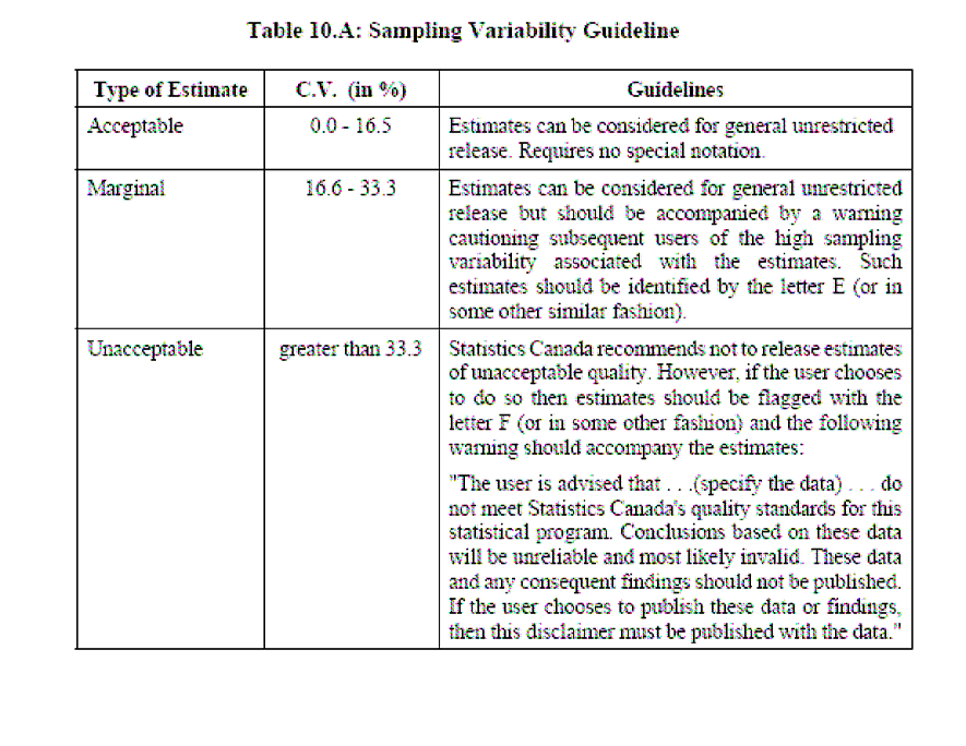
262 243

263 B.2 NPHS selected questionnaires 244

264 245

265 246

266 247

267 248

268 249