Evaluating the value of the option to build a new transmission line under demand uncertainty. Jay Sandeep Ghodke

Transcription

1 Evaluating the value of the option to build a new transmission line under demand uncertainty by Jay Sandeep Ghodke A creative component submitted to the graduate faculty in partial fulfillment of the requirements for the degree of MASTER OF SCIENCE Major: Industrial Engineering Program of Study Committee: Kyung Jo Min, Major Professor Gary Mirka The student author, whose presentation of the scholarship herein was approved by the program of study committee, is solely responsible for the content of this creative component. The Graduate College will ensure this creative component is globally accessible and will not permit alterations after a degree is conferred. Iowa State University Ames, Iowa 2022 Copyright Jay Sandeep Ghodke, All rights reserved.

2 ii DEDICATION I dedicate my work to my family for their constant support. I express my gratitude towards my parents whose words of encouragement and push for determination ring in my ears. I also dedicate this work to my friends who have helped me throughout the process, and I will always appreciate all they have done for me to reach this goal. I dedicate this work to my major professor, research group and colleagues who helped me with the development of my research and providing me with insightful knowledge to overcome any obstacles.

3 iii TABLE OF CONTENTS LIST OF FIGURES...v LIST OF TABLES... vi ACKNOWLEDGMENTS... vii ABSTRACT... viii CHAPTER 1. INTRODUCTION...1 CHAPTER 2. MODEL BACKGROUND...5 OPTIMAL POWER FLOW... 5 Introduction... 5 OPF Model... 6 DCOPF Model... 6 Assumptions... 7 LOCATIONAL MARGINAL PRICES... 7 Introduction... 7 THREE-BUS NETWORK MODEL... 8 DCOPF Model with Transmission Limits DEMAND LATTICE Introduction Binomial Lattice Parameters CASE STUDY Case 1 No new transmission line Demand Lattice OPF Model Formulation Excel Solver Results and Discussion Case 2 New transmission line added OPF Model Formulation Results and Discussion CHAPTER 3. REAL OPTIONS ANALYSIS...27 Introduction Economic Consequence Net Benefit and Total Benefit Exercise Value, Hold Value and Option Value Summary CHAPTER 4. DISCUSSION...33 AC Optimal Power Flow Introduction Page

4 iv LMP Calculation using ACOPF Power Losses in Transmission Line CHAPTER 5. CONCLUSION AND FUTURE SCOPE...38 Conclusion Future Scope REFERENCES...40 APPENDIX 1 OPTIMAL POWER FLOW AND LOCATIONAL MARGINAL PRICE...42 Power Flow Equations Optimal Power Flow using DC power flow equations DCOPF in Linear Programming Solution LMP Calculation using DCOPF APPENDIX 2 EXCEL SOLVER FOR ECONOMIC DISPATCH WITH OPF USED FOR CHAPTER 2 SECTION...50 Excel Input and Output... 50

5 v LIST OF FIGURES Page Figure 1. Three Bus Network Model... 9 Figure 2. Binomial Lattice Figure 3. Binomial Lattice with Risk-Neutral Probability Figure 4. Demand lattice for time period = 6 years Figure 5. Case 1 Network Model Figure 6. Single Period Binomial Lattice Figure 7. Case 2 Network Model Figure 8. Framework of ROA Figure 9. Option Value Lattice Tree... 31

6 vi LIST OF TABLES Page Table 1. Case 1 - LMPs Table 2. Load 1 = MW Table 3. Load 1 = 200 MW Table 4. Load 1 = 270 MW Table 5. Case 2 LMPs Table 6. Load 1 = MW Table 7. Load 1 = 200 MW Table 8. Load 1 = 270 MW... 25

7 vii ACKNOWLEDGMENTS I would like to thank my major professor, Dr. K. Jo Min and my committee member, Dr. Gary Mirka, and Dr. Cameron MacKenzie for their guidance and support throughout the course of this research. I would like to thank Gazi Nazia Nur for her help in lattice excel models. In addition, I would also like to thank my friends, colleagues, the department faculty and staff for making my time at Iowa State University a wonderful experience. I want to also offer my appreciation to those who were willing to participate in my results and observations, without whom, this work would not have been possible.

8 viii ABSTRACT A transmission expansion project is inherently challenging given the large-scale capital commitment needed and the complexity of electric power flow given various uncertain factors ranging from supply and demand as well as cost and price. Hence, it is highly desirable to economically quantify the option/right/permit value to construct a transmission project under uncertainty. Towards this aim, in this paper, we formulate and solve a real option problem to quantify such a construction option when demand shows volatility over time. Specifically, our paper assumes that the demand follows a geometric Brownian motion (gbm) process and shows how the value of the construction option of a transmission line can be derived based on the optimal thresholds of demand to construct or to wait given the optimal power flow calculations and the resulting locational marginal prices. The key features of our model and analysis are illustrated via an extensive numerical example. In particular, this framework shows the economic ramifications of using locational marginal prices as a performance criterion.

9 1 CHAPTER 1. INTRODUCTION With the deregulation movement of the 1990s, the electricity industry evolved from a controlled, vertically integrated, local monopoly to one where it is dominated by competitors producing electricity while the transmission grids are maintained by the utilities (Slocum, 2008). As a result, the transmission and the generation facets of the electric power industry have been separated; for instance, the generation unit's decisional authorities are not obliged to provide power while the network owners have to confront the ever-increasing demand while keeping the technical necessities under control. The power generation sections essentially became competitive activities while the transmission section were still controlled monopolies. The primary reason for reorganizing the industry has been to boost the power generation competition and offer a choice for the consumers to select the power distributor so that the electricity distribution s economic efficacy will be improved. This deregulation permitted power companies to sell electricity at the maximum possible cost, whereas under the original model, power prices were directly linked to generating costs combined with an acceptable and controlled profit margin. The transmission network must be developed in the most cost-effective approach that will suffice the requirements of power producers and end-users while maintaining the reliability factor. The network owners also determine expansion planning of the network like adding new transmission lines or power generation centers based on the frequency of congestion. Thus, regulatory bodies face the necessity to offer incentives to build technologically and financially efficient networks under a market environment (Wu, et al., 2006). Moreover, the transmission system works as the backbone of the electric power industry, and hence incentives must be provided to take timely decisions on transmission expansion planning, which will enhance

10 2 economic efficiency and reduce generation dispatch costs. Since the power demand is highly uncertain and volatile, these factors play a significant role while evaluating transmission investments. Moreover, the increase in policies that encourage generation from renewable sources has further increased volatility in the power supply due to the uncertainty in the availability of renewable energy sources. All these factors pose a challenge to the transmission expansion planning given that they are responsible for meeting the uncertain and increasing demands while maintaining the technical requirements, optimality, and stability of the system. Future uncertainties can be accounted for from numerous sources. For instance, demand growth has been one of the primary sources of future uncertainties. The ambiguity in demand varies due to multiple factors, including the location, season, daily usage, and these operational impacts must also be considered in transmission expansion planning. Additionally, given the irreversibility aspect of the expansion plans, network owners know that developing projects based on deterministic futures can be financially consequential if the future is different than what it was considered during planning. Hence, it is irrational to plan on a single deterministic future given the uncertainty in cost of fuel, federal regulations, and unanticipated technological advancements (Olatujoye, 2015). For instance, factors like world politics, climate change, can change the cost of fuel drastically. Ultimately, uncertainty becomes one of primary factors in evaluating transmission expansion planning projects. And so, the authorities require flexible financial methodologies that can emphasize uncertainty as well as the risk to value the transmission expansion plans (Pringles, et al., 2014). Real option analysis (ROA) is a conceptual application of financial options theory (Black & Scholes, 1973) that is applied to physical or real assets. According to financial options theory, the owner has the authority but not the compulsion to execute financial decision at a particular

11 3 cost. Consequently, an owner who makes calculated investment has the authority, but not the compulsion, to profit from these possibilities in the future. As a result, this methodology safeguards the owners from unexpected risk while not constraining revenue gains. Owners may use real options analysis to assess alternatives for effectively managing calculated investments from a wider viewpoint (Myers, 1984). Programs, strategies, and variable financial investments can all be considered as real options. These options may also include delaying, growing, downsizing, or even terminating the investment endeavors. Other real options include updating the equipment, modifying the purpose, or increasing the project life cycle. Some options emerge organically. Others may be calculated investments or developed at a specific cost. ROA is a financial tool developed for evaluating large-scale, irreversible investment plans that offer managerial flexibility in strategy-making under uncertainty (Avinash & Robert, 1994). In this work, we consider the transmission expansion plans as strategic real options and since they characterize the above-mentioned factors and hence, we can implement real options analysis to evaluate the plans under uncertainty. We develop a framework for valuing the transmission expansion projects based on ROA which will allow the network owners to effectively analyze multiple options with regard to the decision of when to execute the plan given that they would execute it. This approach evaluates the parameters value of the regulatory framework design for merchant transmission in order to deliver fast and reliable signals to encourage power network infrastructure expansion. This work puts forward the framework for evaluating transmission expansion options for the network owners under uncertainty. The framework is fundamentally based on demand evolution and the locational marginal prices (LMPs) obtained by solving the optimal power flow (OPF) problem. Furthermore, we show that the values of the expansion plan can be determined if

12 4 they were to advance or postpone the project. We also assume that the demand evolution follows a geometric Brownian motion process. The transmission expansion plan considered in this work is to add a new transmission line in the three-bus model parallel to an existing line which is described in the later section. The remainder of the paper is structured as follows. First, we present the background on optimal power flow problems based on DC power flow equations and the calculation of locational marginal prices. Next, we explain the three-bus network model developed for a comprehensive numerical case study and describe the two cases that help demonstrate our framework's vital characteristics. Then, we present the numerical results, including the valuation of the option using ROA. Later, we discuss ACOPF model formulation and the factors affecting power transmission losses. Finally, we conclude the paper with a summary and future scope.

13 5 CHAPTER 2. MODEL BACKGROUND This chapter talks about optimal power flow (OPF) and the DC approximation of the OPF. After that, we discuss in brief the locational marginal prices (LMPs) and the factors affecting the LMPs. Next section describes the three-bus network model in detail along with the introduction of the two cases and DCOPF model for this network. In the next section, the demand lattice is explained to illustrate the evolution of the demand. Finally, the last section is case study on the three-bus model with two different cases and multiple scenarios followed by its results and discussion. OPTIMAL POWER FLOW Introduction Optimal power flow (OPF) is an optimization model which aims at determining the most efficient production of power to meet the total demand in the network while reducing the total costs. OPF includes the Economic Dispatch (ED) model with equations that simultaneously solve ED and optimal power flow. The ED model obtains the lowest-cost power generation within the generators' physical generation limits. Only difference between OPF and ED is that OPF combines ED and power flow problems. Nevertheless, ED neglects various details like the effects of the generation on the transmission system. The objective function of the OPF model is the same as that of ED, i.e., to minimize the total generation cost, which is subjected to a set of constraints that include nodal power balance equation, generator limit equation, transmission limit equation, and power flow equation. The OPF problem can be modeled for both AC and DC networks, but ACOPF model is significantly more complex than the DCOPF due to its non-linearity, convexity, and high computational time. Hence, DCOPF is generally implemented where time-sensitive decisions

14 6 and analyses are to be delivered. DCOPF is derived from the DC power flow equations, which neglect the reactive part from the AC power flow equations. Therefore, DCOPF is a linear programming method that linearizes and approximates the ACOPF as direct current (DC). The rest of this section discusses OPF model, DCOPF model formulation, and the constraints added to it. OPF Model (Wood, et al., 2014) describes the objective function of the OPF as to minimize the total generation cost while supplying power to the total demand in the network. This is achieved by dispatching power from the cheapest generator and then moving on to the next generator when the limit is reached, or congestion is caused in the network causing violation of transmission limits. DCOPF Model The AC power flow is more complicated and has more complex equations which makes it arithmetically difficult to solve the optimization problem. Therefore, we use DC power flow to model the OPF problem with constraints. The AC power flow can be approximated using DC power flow which makes it easier to solve the optimization problem due to its less complexity. DCOPF is particularly helpful in network analysis of renewable energy sources which generate DC power (Stott, et al., 2009). We consider the following assumption to model the DCOPF problem. These assumptions are fundamental for solving the DC approximation of the OPF model. They are based on the three bus model network cases.

15 7 Assumptions 1. The resistance (R) in the transmission lines is negligible compared to the reactance (X). Because the resistance of each branch, is so little in comparison to the branch reactance, it can be set to zero. 2. The value of the voltage magnitude (V i ) is equal to The difference between the voltage angle θ i θ j between in transmission line is negligible that cos (θ i θ j ) = 1 & sin (θ i θ j ) = θ i θ j 4. Bus 1 is assumed to be the reference bus or slack bus. It implies that phase angle of bus 1 will be There is no upper limit to the power generation capacity of the generators. 6. The losses in the transmission system are negligible. After the introduction of optimal power flow and its DC approximation followed by the assumptions considered for this model, we move on to LMPs and the factors affecting it. LOCATIONAL MARGINAL PRICES Introduction The Locational Marginal Price (LMP) of any bus is the minimum cost of electrical power required to meet the additional demand of that bus. LMP determines energy pricing in real-time at sites throughout the local high voltage transmission system. LMP is a vital element in aggressive wholesale market transactions (Liu, et al., 2009). LMP also reflects the cost of congestion and transmission losses across the network. Therefore, it includes three main factors which decide the value of LMP in real-time. These prices serve as real-time, ever-changing benchmark signals for buyers and sellers in wholesale power markets. They advise decisions about infrastructure investment, help encourage grid

16 8 reliability, and aid network owners to provide competitive markets for the most economical and reliable sources of power. (Wood, et al., 2014) Cost of Generation This cost is denoted by the power generators which include primary parameters like fuel cost. The generation cost of these generators which provide their power to the network includes this cost and the production cost. Usually, the most reliable and economically beneficial power is bought by the network owners. Cost of Congestion The network is usually designed to supply enough power to all its buses including a surge of demand up to a certain level. During low demand situations the power can transmitted through the network without restrictions. Whereas in the high demand situations the power flow can be restricted by physical constraints of the transmission network or the generation limit. The network owners utilize high-cost generation leading to increased LMP. Transmission Losses Power lost in transmission can be around 5% (PJM, 2020) of the total power. This is related to the physical properties of the transmission lines and environmental factors like high ambient temperature causes power loss by convection. Copper losses also contribute majorly towards the power lost in transmission. THREE-BUS NETWORK MODEL This three-bus network model is a simplified version from the numerical example solved in the textbook Power Generation, Operation and Control by (Wood, et al., 2014) on page 356.

17 9 This test bed is also similar to the test bed used by (G. Nazia, et al., 2021) in her doctoral dissertation which extends this research work by adding a new generator to the 3-bus model instead of transmission line as power expansion project. Figure 1 represents a 3-bus network which consists for demand loads at all 3 buses and generators at bus 2 and bus 3 only. Assume there is no upper limit to the generation capacity of the generators. The marginal cost of generator 2 is 7.85 $/MWh and generator 3 is 7.97 $/MWh. The load at bus 1, bus 2 and bus 3 is 200 MW, 550 MW and 100 MW respectively. The buses are connected with each other via transmission lines. Reactance for line 1-2, 1-3 and 2-3 is 0.1 PU, PU and 0.2 PU, respectively. The line 1-2 has a transmission limit of 210 MW. That means, only 210 MW can be transmitted from bus 1 to 2 or the other way round. Other transmission lines do not have any transmission limit. Figure 1. Three Bus Network Model The total demand in the network is 850 MW. DCOPF will be used to obtain the optimal generation by each generator to minimize the total production cost. The DCOPF will give the

18 10 LMP at each bus and the power flow between all the buses. The objective function of minimizing the production cost is subjected by the generation limit, nodal power balance equation and generator load balance equation. Consider two cases and each case will have 3 scenarios. Case 1 In case 1, the 3-bus network will have the originally presented transmission system with transmission limit of 210 MW between bus 1 and 2. The 3 scenarios will be varying the bus 1 demand load. In scenario 1 the demand at bus 1 will be MW, scenario 2 will have 200 MW and scenario 3 will have 270 MW. Case 2 In this case, a new transmission line will be added to the network between bus 1 and 2 parallel to the existing transmission line 1-2. This new transmission line will be imposed with transmission limit. The three scenarios will be repeated for Case 2 as well. DCOPF Model with Transmission Limits In this section the DCOPF model is presented with addition of the transmission limit constraint. The DCOPF problem is solved with the new set of constraints and the LMPs are obtained for all the buses. Specifically, MC i = marginal cost of node i G i = generator at node i θ i = phase angle for node i P ij = Power-flow in line i-j P load i = demand load at node i Objective Function:

19 11 min (MC 1 *G 1 + MC 2 *G 2 ) Decision variables are G 1, G 2, G 3 and θ 1, θ 2, θ 3, and P 12, P 13, P 23 and P load 1, P load2, P load 3 and P total load Subject to following constraints: Generator limit inequality constraint: There is no maximum generation limit to the generators i.e., the generation is nonnegative. G i 0, i = 1, 2, 3. Generator load balance equality constraint: P total load (G 1 + G 2 ) = 0 Where, P total load = P load 1 + P load2 + P load3 P load 1 = 200MW, P load2 = 550MW, P load3 = 100MW Nodal power balance constraints: 100[B x ]θ i = P i P loadi Where, B ij is the susceptance of the branch i to j given by: B ij = ( 1 x ij ) x ij = reactance between line i and j Reactance for line 1-2, 1-3 and 2-3 is 0.1 PU, PU and 0.2 PU, respectively. Power-flow in each branch: Transmission limit constraints: P ij = 100 B ij (θ i θ j ) = 100 θ i θ j x ij

20 θ i θ j x ij P ijmax 100 θ j θ i x ij P ijmax To solve the DCOPF model, Excel Solver is used as an optimization tool. The SOLVER add-in helps solve the optimization problem with the objective function as minimizing the total generation cost. Solving the model using Simplex-LP or GRG-Nonlinear method in solver, the DCOPF results are obtained. The LMP of each bus can be obtained from the sensitivity report obtained after solving the DCOPF problem. The sensitivity report gives the value of the Lagrangian multiplier. This multiplier denotes the LMP of that particular bus. DEMAND LATTICE Introduction Option value evaluation based on geometric Brownian Motion (gbm) process which is a continuous stochastic process is very hard to compute. Hence, using a discretized form will be less complex for such type of a process. A binomial lattice model is constructed to indicate the uncertain demand evolution. We only consider the demand evolution for bus 1 in our case study presented in the next chapter for process simplification. The evolution of demand at this bus is assumed to follow gbm. Binomial Lattice Parameters (Cox, et al., 1979) created one of the most frequently used binomial lattice model. (White, 2016) also explained the construction of binomial lattices in his paper. This method states that a variable D has two options for the next period; to go up or go down. D goes upwards by an up-factor u and goes downwards by a down-factor d. The probabilities of going up or down are p and (1 p) respectively.

21 13 Figure 2. Binomial Lattice The up factor and the down factor can be calculated using the following equations: u = e σ Δt d = 1 u = e σ Δt Where, Δt is the length of time period and σ denotes the volatility of the process. The probability p used here is not a risk-neutral probability (K. Jo & Fikri, 2018). For binomial lattice construction we require risk-neutral probability q instead of p since p is derived by discretizing the gbm process hence, it is not risk-neutral. In real options analysis, cash flow is discounted at a risk-free discount rate (r f ) while the cash flow probabilities are altered with risk. Risk-neutral probabilities can be obtained by using the following equation: q = er f d u d The binomial lattice with risk free discount rate is illustrated below. D (0,0) denotes the initial demand at time 0. Variable D (0,0) has two possibilities, i.e., it can go either up or down in the subsequent period with risk-neutral probability q and (1 q) and up factor (u) or down factor (d). Figure 3 shows the binomial lattice model for two time periods.

22 14 Figure 3. Binomial Lattice with Risk-Neutral Probability Now considering Figure 1 along with the same parameters, we construct the binomial lattice model for demand at bus 1 assuming that the demand evolution at bus 1 follows gbm. The initial demand at bus 1 is 200 MW. The economical gain of adding a transmission line in the network is discounted with a risk-free discount rate of % compounded continuously per annum. The volatility (σ) of the power demand is assumed to 30% per year. Therefore, we can determine the values of up-factor (u), down factor (d), and risk-neutral probability (q). The length of a single time period Δt is assumed to be 1 year. The increase and decrease in demand can be calculated by: D (t,i) = u D (t 1,i 1) or, D (t,i 1) = d D (t 1,i 1) The demand lattice shown in Figure 4 is modeled for a time period of 6 years which is equal to 6 time periods, as single time period Δt is 1 year.

23 15 Figure 4. Demand lattice for time period = 6 years CASE STUDY Case 1 No new transmission line As implied from the three-bus model network section, this Case 1 is also shared with Nazia s doctoral dissertation (G. Nazia, et al., 2021). In the first case study, the three-bus network will have the originally presented transmission system. Accordingly, a transmission limit of 210 MW between bus 1 and 2 will be imposed, which means that the transmission line between bus 1 and 2 can transmit up to 210 MW. Remaining transmission lines have no physical constraints. As seen in the Figure 1, there are three buses connected to each other. There are two generators at bus 2 and 3. It is assumed that there is no upper bound to the generation capacity of these generators. The marginal cost of generator 2 is 7.85 $/MWh and generator 3 is 7.92 $/MWh. These costs represent the cost of producing an additional unit of electricity. The demand load at bus 1, 2 and 3 is 200 MW, 550 MW and 100 MW respectively.

24 16 Figure 5. Case 1 Network Model Demand Lattice From previous section we have the following demand lattice for initial single time period. The initial demand for the demand lattice is load at bus 1, i.e., 200 MW. Figure 6. Single Period Binomial Lattice In the demand lattice, 200 MW represents the starting of the period 0 and MW or 270 MW show the starting of the period 1. Here we note that (p, s) indicate the period and state

25 17 in the demand lattice. Thus, D (p,s) indicates the demand load value at period (p) and state (s). Therefore, we have D (1,1) = 200, D (2,1) = 270, D (2,2) = These 3 values denote the three scenarios and for each scenario OPF will be calculated. OPF Model Formulation In the case study, the problem is solved using OPF methodology wherein the objective function is to minimize the production cost which is subjected to certain constraints. Moreover, this methodology is more innate for a small illustration like this where we try to make the OPF problem less complex to understand the concept and utilize it for the real option analysis. Since the transmission networks use alternating current (AC), ACOPF method is used to model the OPF problem which considers the AC complexities. Nevertheless, ACOPF is a nonlinear, nonconvex and an intricate optimization problem which requires more time to solve. Current models need to be quick in turn to be pragmatic for real-time analysis. Therefore, a linear programming method called DCOPF is used which basically is the linearization and approximation of the ACOPF as direct current (DC). The LMP is calculated by obtaining the value of Lagrangian multiplier. As discussed in the previous section, it is assumed that the losses in the transmission system are negligible; reactive power is neglected; and resistance negligible compared to the reactance. To obtain the LMPs at different nodes, the DCOPF is solved. Specifically, MC i = marginal cost of node i G i = generator at node i θ i = phase angle for node i P ij = Power-flow in line i-j P load i = demand load at node i

26 18 Objective Function: min (MC 3 *G 3 + MC 2 *G 2 ) Decision variables are G 2, G 3 and θ 1, θ 2, θ 3, and P 12, P 13, P 23 and P load 1, P load2, P load3 and P total load Subject to following constraints: o Generator limit inequality constraint: There is no maximum generation limit to the generators i.e., the generation is nonnegative. G i 0, i = 2, 3. o Generator load balance equality constraint: P total load (G 1 + G 2 ) = 0 Where, P total load = P load 1 + P load2 + P load3 P load 1 = 200MW, P load2 = 550MW, P load3 = 100MW o Nodal power balance constraints: 100[B x ]θ i = P i P loadi Where, B ij is the susceptance of the branch i to j given by: B ij = ( 1 x ij ) x ij = reactance between line i and j Reactance for line 1-2, 1-3 and 2-3 is 0.1 PU, PU and 0.2 PU, respectively. We use a per unit (PU) system to bring uniformity in the system values by absorbing large differences in absolute values by converting them into simplified base relationships. All values are expressed as

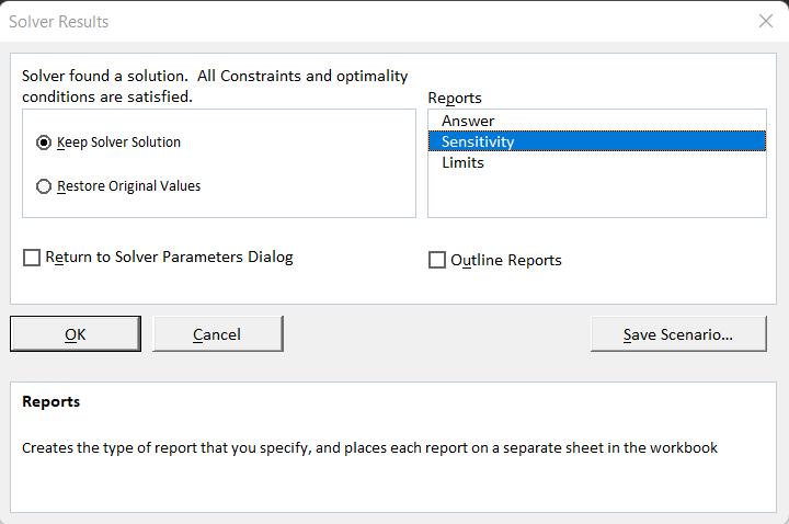
27 19 fractions of a defined base value. The base power is usually chosen as a convenient round number such as 10 MVA or 100 MVA. The base power can be any arbitrary number or the highest rating of a component in the system. For instance, let us consider a generator which has a rating of 150 MWh and the system base power as 100 MVA. If the generator produces 120 MWh, then it is equivalent to 1.2 PU in per unit system. o Power-flow in each branch: P ij = 100 B ij (θ i θ j ) = 100 θ i θ j x ij o Transmission limit constraints: 100 θ i θ j x ij P ijmax 100 θ j θ i x ij P ijmax Excel Solver To solve the DCOPF model, Excel Solver is used as an optimization tool. The SOLVER add-in helps solve the optimization problem with the objective function as minimizing the total generation cost. Solving the model using Simplex-LP or GRG-Nonlinear method in solver, the DCOPF results are obtained. The LMP of each bus can be obtained from the sensitivity report obtained after solving the DCOPF problem. The sensitivity report gives the value of the Lagrangian multiplier. This multiplier denotes the LMP of that particular bus. The procedure for the Excel Solver modelling is presented in Appendix 2 Excel solver for economic dispatch with OPF.

28 20 Results and Discussion Table 1. Case 1 - LMPs Scenario Load (MW) LMP 1 ($/MWh) LMP 2($/MWh) LMP 3 ($/MWh) Table 2. Load 1 = MW Generator Generation (MW) Transmission Line Optimal Power Flow (MW) Table 3. Load 1 = 200 MW Generator Generation (MW) Transmission Line Optimal Power Flow (MW)

29 21 Table 4. Load 1 = 270 MW Generator Generation (MW) Transmission Line Optimal Power Flow (MW) In the first case we have a transmission line limit of 210 MW on line 1-2. When the load is MW at node 1 (Scenario 1), generator 2 dispatches power to all the buses. This is because the generator 2 has cheapest marginal cost compared to generator 3. Therefore, the DCOPF model uses G2 to meet all the demand load. The power flow between line 1-2 is MW which is less than the transmission limit and hence the constraint is not violated. Similarly, G2 meets the total demand when the load at bus 1 is 200 MW (Scenario 2). In both these scenarios, the LMP at all the nodes will be the marginal cost of G2 since if an additional unit of power is needed, it will be met by G2 without violating the transmission limit. Therefore, the LMP at bus 1, 2 and 3 is 7.85 $/MWh. In Scenario 3, when the load is 270 MW at bus 1, the DCOPF algorithm initially opts for G2 to satisfy the total demand. But the power flow in line 1-2 violates the transmission limit. The total demand cannot be satisfied by G2 alone. Hence, the DCOPF model selects the next cheapest generator to contribute to the total demand. G3 contributes to the remaining load while G2 produces the maximum amount to reduce the total production cost. With the cheapest MC of 7.85 $/MWh, G2 will be producing MW and out of that 550 MW is used by bus 2 itself to meet its demand. Since line 1-2 has the transmission limit imposed, 210 MW is transmitted to bus 1. The remaining 67.5 MW is transmitted to bus 3. Bus 1 still has 60 MW of demand load unmet. Due to Kirchhoff s law, G2 cannot send more power to bus 1 or bus 3 without violating

30 22 the transmission limit imposed on line 1-2. Therefore, G3 produces the remaining 92.5 MW to meet the total demand of the network MW is used by bus 3 itself and 67.5 MW from G2 meets the demand at bus 3. As result, the demand is met by G2 and G3, and any additional demand at bus 3 can be met G3 and hence, the LMP at bus 3 is the marginal cost of G3, i.e., 7.97 $/MWh. Since Bus 1 does not have a generator, the remaining load must be met by G2 and G3 as well. As a result, the LMP of bus 1 is combination of marginal costs of G2 and G3 which $/MWh. The amount of the power transferred by each generator can be determined using the power transmission distribution factors (PTDFs). Hence, these LMPs are calculated using the percentage of power transferred by each generator to that bus. Case 2 New transmission line added In the second case study, the 3-bus network will be modified by adding a new transmission line between buses 1 and 2 and using Case 1 as a reference example. We assume that the new transmission line will be added at the beginning of period 0 from the demand lattice. The transmission limit of this new line is 105 MW, and the reactance is half of that of the original line between bus 1 and 2. In the previous case, when load at bus 1 reached 270 MW, then both the generators come into action which increases the generation cost of the network. In this case, DCOPF is solved with a new transmission line while the other parameters remain the same. Figure 3 shows the addition of new transmission line between buses 1 and 2.

31 23 Figure 7. Case 2 Network Model Since the demand evolution is assumed to be same as in Case 1, there will be three scenarios which will denote the demand values at bus 1 as MW, 200 MW or 270 MW. OPF Model Formulation The DCOPF model described in the previous case will be used for Case 2. While programming the DCOPF model for Case 2, the capacity of the transmission lines between buses 1 and 2 will be added linearly. Thus, the total transmission capacity between bus 1 and 2 is 315 MW. According to M. Wang in (Wang, 2010), the equivalent impedance (Z) in two parallel lines in an AC network is given by the following equation. Z eq = Z 1Z 2 Z 1 + Z 2 Impedance (Z) consists of real and imaginary terms and is denoted as Z = R + jx, where R is the resistance (real part) and X is the reactance (imaginary part). But we have assumed that

32 24 the resistance is negligible compared to the reactance in the network and hence impedance (Z) is equal to the reactance (X) in the network. Therefore, from the above equation, reactance of the lines can be obtained using the following equation which denotes the equivalent reactance of two parallel lines. X eq = X 1X 2 X 1 + X 2 Where, X eq denotes the equivalent reactance between two parallel lines and X i is the reactance of line i = 1, 2. Results and Discussion Table 5. Case 2 LMPs Scenario Load (MW) LMP 1 ($/MWh) LMP 2($/MWh) LMP 3 ($/MWh) Table 6. Load 1 = MW Generator Generation (MW) Transmission Line Optimal Power Flow (MW)

33 25 Table 7. Load 1 = 200 MW Generator Generation (MW) Transmission Line Optimal Power Flow (MW) Table 8. Load 1 = 270 MW Generator Generation (MW) Transmission Line Optimal Power Flow (MW) In the second case, we have a new transmission line between bus 1 and 2 with a limit of 105 MW parallel to the existing original line between line 1-2. For Scenarios 1 and 2, the optimal power flow and the generation dispatch will be similar to Case 1. Also, the capacity between bus 1 and 2 has further increased which allows more power to be transmitted between the two buses. In Scenario 3, when the load is 270 MW at bus 1 and after solving the DCOPF problem we see that G2 meets the demand of whole network without violating the transmission constraint. As compared to Case 1 where G2 cannot meet the whole demand due to the limit imposed on line 1-2. Any additional unit of electricity for all the buses can be provided by G2 itself without violating the transmission limit and hence the LMP for all buses will be the marginal cost of G2, i.e., 7.85 $/MWh. This is achieved due to the new transmission line being

34 26 added in the network between bus 1 and 2. The line is strategically added at the point of congestion to relieve it and achieve the most economic generation dispatch.

35 27 CHAPTER 3. REAL OPTIONS ANALYSIS Introduction We utilize real options analysis (ROA) in this research to determine the option value of installing a new transmission line. ROA was used by several researchers in power systems, in (Blanco, et al., 2012); a method to value the option of deferring transmission line investments while obtaining flexibility by investing in flexible AC systems was demonstrated. (K. Jo & Fikri, 2018) proposed framework to evaluate the value of the option to expand the network under major and difficult financial and governing uncertainties. The proposed methodology in this paper assumes: 1. The power demand follows geometric Brownian motion. 2. The new transmission line is functional at the same period the installation decision is made. 3. Initial demand, power flow and physical limits of transmission lines are known. 4. The expansion decision is made from the point of view of a particular community. The framework used in this research for evaluating the value of the option of adding a transmission line is given in Figure 5. First, according to our assumption that the electricity demand follows a geometric Brownian Motion, we construct a demand lattice for a period of 6 years. This lattice is modelled using the discrete time binomial lattice method. The calculation and modelling of demand lattice is shown in the section Demand Lattice of Chapter 2. We start with addressing the uncertainty in electricity demand and map demand for the modelling horizon using binomial lattice. Since electricity demand in volatile and uncertain, binomial lattice model is an appropriate option for this problem. Next, we calculate the economic benefit of adding a new transmission line to the network (Case 2) and compare it with the original network (Case 1)

36 28 with no new transmission line. The network and its modification for both the cases has been explained in detail in Chapter 2. Mapping demand over the modelling horizon using a binomial lattice Calculating the cost paid by the community at bus 1 to fulfil their electricity demand based on the locational marginal price for case 1 and 2 Computing the net benefit by subtracting the cost of case 1 from case 2 Evaluating the exercise value and hold value at the end period, then determining the option value as max(exercise value, hold value) Determining the option value at time 0 by repeatedly calculating the expected value and discounting it Figure 8. Framework of ROA In the next step we determine the net benefit which is the difference between the economic benefit of Cases 1 and 2. Next, we determine the option value at the end of the period and then finally obtain the option value at initial demand by continuously calculating expected value and discounting it. Economic Consequence In Chapter 2, we obtained the demand evolution at bus 1 for time period of 6 years. The OPF model and LMPs calculation methodology is presented in Chapter 2 for both the cases with demands from time period 0 to 1. The LMPs for the rest of the loads from the demand lattice can be calculated similarly. The economic consequence of bus 1 for 1 time period (1 year) can be obtained using LMP and demand at bus 1, shown in following equations.

37 29 K j t,i = D t,i LMP j t,i 8760 Here, K j t,i represents the annual cost required to meet the electricity demand at time period t = 0,1,2,.. and at state i = 0,1,2,.. And, j = 1,2 represents the case number. Therefore, using the above equation the economic consequence for both the cases can be obtained. The values shown are in million USD. Net Benefit and Total Benefit K 1 t,i = = K 2 t,i = = The net benefit (B t,i ) of adding a transmission line in the network can be determined from the difference between the economic consequences of Cases 1 and 2. In other words, the difference between the two values tells us if the adding a transmission line to the original network will be beneficial to the network or not. (The value shown are in million USD). B t,i = K 1 t,i K 2 t,i = B t,i denotes net benefit at time period t and at i th state. The expected value of total benefit (EV t,i ) can be obtained using risk free interest rate (e r f) and risk neutral probability (q) along with net benefit. It can be obtain using following equation: EV t,i = B t,i + [q B t+1,i+1 + (1 q) B t+1,i ] e r f Exercise Value, Hold Value and Option Value Installing a new transmission line can be considered as a real option since it requires a significant investment and is irreversible. This is similar to an American call option where the decision-maker can exercise the option at any moment before it expires (Ramanathan & Siri, 2006). The option value (OV t,i ) of an American option is calculated using the option's hold value

38 30 (HV t,i ) and the option's exercise value (XV t,i ). Initially the hold and exercise values of the last time period is determined. The hold value reflects the expected value of the option if it is not exercised today and is kept for a longer length of time. However, the hold value at the end of the term is zero since retaining the option will result in no future benefit. Moreover, the exercise value of the last period denotes economical gain from adding a transmission line. XV t,i = EV t,i K Here XV t,i represents the exercise value at time period t and at state i and K is the construction cost of a new transmission line which is assumed to $100,000 for this model. The HV t,i will be 0 at last period. Option value (OV t,i ) at the end period is the maximum value between exercise value and hold value. (OV t,i ) = Max(EV t,i, HV t,i ) The hold value is calculated backwards from the end period. It can be calculated using (OV t,i ), risk neutral probability and risk-free interest rate. HV t,i = [q OV t+1,i+1 + (1 q) OV t+1,i ] e r f Finally, the option value at the initial demand can be obtained by calculating values from end period to the first period. Therefore, the option value lattice can be constructed using the demand lattice from Chapter 2. Figure 6 represents the option value lattice model for 6 time periods. The first number is total benefit, representing the summation of present benefit and expected future benefit of adding a generator at that time period. The second number is exercise value, which is the projects intrinsic value if exercised at that time period. The third number is hold value. Hold value at a time period depicts the value of the option if it is not exercised at that time period and being held for one more time period. Finally, the last number is the option value, which is the maximum number between the exercise value and hold value at that time period.

39 31 Furthermore, the optimal timing of adding a generator depends on demand movement. We can see from Figure 5, if demand goes upward after one time period, then exercising the option at time 1 is optimal. On the other hand, if demand decreases at time 1, exercising the option after two upward demand movements will be optimal. That means exercising at time 3 will be optimal. Figure 9. Option Value Lattice Tree

40 32 Summary The real options analysis can be efficiently used as a financial tool which provides flexibility and managerial insight. With the help of ROA, the investment planners can understand the effects of executing expansion plans and whether it will benefit if executed now or in the future. In this numerical case study, we saw that when the demand is high, it leads to congestion in the network which brings in power from expensive generators. This ultimately increases the LMPs, and total generation cost and the consumers end up bearing this cost. Nevertheless, with the help of ROA and OPF, the transmission expansion planners can determine the value of expansion options given that the owners will do it and when they do it. This analysis provides an insight into the valuation of the project and the decision whether it should be executed now or in the future. For instance, from Figure 9 it is evident that the value of the option when the demand is high (270 MW) is higher compared to when the demand is low (148 MW). This is due to the congestion in the network being relieved by executing the option (in this case adding a transmission line) which reduces the LMPs and total generation cost. Whereas the option value is less when the demand is low because adding a new transmission line will not improve the power flow or reduce the LMPs hence, it is not a logical option during that stage. Moreover, we also see that the LMP at bus 3 also reduces when the transmission line is added between buses 1 and 2. This implies that, the expansion plan not only benefits the community at bus 1 but also the community at bus 3. The LMP reduction occurs because the cost of power production of the generator at bus 3 is more expensive than the generator bus 2 and hence in Case 1, (no new transmission line added) the total production cost increases along with the LMP at bus 3 since generator 3 also produces power to meet the total demand in the network.

41 33 CHAPTER 4. DISCUSSION AC Optimal Power Flow Introduction The entire electrical network is essentially alternating current (AC) power flow. ACOPF model is formulation of optimal power flow using AC power flow equations. This method is more capable and dependable compared to DCOPF. Federal Energy Regulatory Commission (FERC) has stated that if ACOPF based software is used by today s electricity market then it could potentially avoid billions of dollars annually. In contrast to DCOPF, ACOPF takes into consideration current, voltage, reactive power, various types of losses which ultimately results in improved accuracy and reliability. But this problem is non-linear and hence very complex in terms of computation and cost-effectiveness. This is mostly due to the problem being nonconvex and including continuous as well as binary functions. Moreover, there is no assurance that optimizer can obtain the global minimum due to the problem s nonconvexity (Barati & Amin, 2017). The network owners need fast calculation methods in order to obtain day ahead and realtime LMPs. Hence, approximations are used to achieve a rational solution to the problem. The accuracy and dependability of such approximated model like DCOPF is relatively lesser compared to the more realistic ACOPF model but the low computational requirements and costeffectiveness of DCOPF model gains more advantage over ACOPF. In this section, ACOPF formulation is described with all the constraints. The credits for this ACOPF formulation are given to (Wood, et al., 2014). The ACOPF model has almost twice as much as variables compared to DCOPF which makes it difficult to solve. The objective function of the model will be the same, i.e., to minimize the generation cost. In ACOPF, both real and imaginary power flow equations are needed.

42 34 Objective Function: The ACOPF can be modelled for various objective functions like generation cost minimization, loss minimization, fuel cost minimization and minimizing generation amount produced. Most commonly, ACOPF is modelled for cost minimizations for electricity generation. Here C i denotes the marginal cost of generator i and P geni is the amount of power generated by generator i. Subject to: Power Flow Equations: N min i=1 C i (P geni ) The power flow equations are derived considering a net complex power injection to a node is given by S i = P i + jq i where P i denotes the real power and Q i denotes the reactive or imaginary power. These power flow equations form the basis of the optimal power flow problem. P i denotes the real power flow flowing out of bus i N P i = V i V k (G ik cos (θ i θ k ) + B ik sin (θ i θ j )) k=1 Q i denotes the reactive power flow flowing out of bus i Generator Limit Inequality: N Q i = V i V k (G ik sin (θ i θ k ) B ik cos (θ i θ j )) k=1 min max P Geni < P Geni < P Geni i N Generator Reactive Power Limit Inequality: min max Q Geni < Q Geni < Q Geni i N

43 35 Nodal power balance equality: The ACOPF optimization problem takes transmission losses into consideration too. Thus, the power balance equation states that the total power generated should be equal to the total load in system plus the transmission losses. N P Geni i=1 = P Total load + P losses N is the total number of generators. Transmission Line Capacity Limit: The real and reactive power flow in the transmission line should less than or equal to the flow limit of the line. Voltage magnitude inequality: P ij = {V i [(V i V j )y ij + V i 2 y ij ]} P ijmax V i min < V i < V i max i = 1.. N Voltage Angle inequality: π < θ i < π i = 1.. N LMP Calculation using ACOPF ACOPF is generally not used in electricity markets for LMP calculations for the reasons stated in the previous sections. To obtain the LMP of each bus, Lagrangian equation is used for this problem. The Lagrangian multiplier is used for the equality and inequality constraints and the optimization is solved. The value of this multiplier gives the LMP at that particular bus.

44 36 Power Losses in Transmission Line In our model we assume that resistance in the network is negligible compared to the reactance. This assumption makes the problem less complex and reduces the time required to solve these problems which is especially beneficial in the day ahead LMP calculation. But this can reduce the accuracy and reliability of the model. For more accurate values and to increase the fidelity of the model, it is recommended to include power losses in the OPF calculation. In this chapter, the types of power losses are described to give an overview and how power loss is included in the optimization model. As the length of the transmission line increases, the power losses also increase. The resistance per miles is relatively very less, but it can have significant effect on long length transmission lines. Increased resistance leads to generation of heat in the conductors which is causes power losses. These losses are called as I 2 R losses or copper losses. I 2 R is the formula used to calculate power losses in the conductor. It is formed by combining Ohm s Law and Power Law equation. Power loss can also be caused due to skin effect, corona discharge and other non-technical factors. The governing factor in copper losses is the resistance of the conductor. Resistance of a transmission line conductor further depends on its length and the cross-sectional area. Following equation illustrates the relation between resistance and length and area of the line. Where, R = ρl A (Ω) R = Resistance in the conductor; ρ = Resistivity; A = Cross-section area (Reta-Hernández, 2012) explains that the transmission cables used in overhead transmission lines use aluminum conductors because of its light weight and low cost with steel reinforcement. They have alternate layers of conductors and reinforcements wound in spiraling

45 37 direction. Opposite direction of spiral wounding is used for consecutive layers to increase the strength of the cable. Such type of manufacturing method is easier compared to a solid cable of same diameter. It also offers better strength-to-weight ratio due to reinforcements. The resistance in such spiraled and bundled cables can be formed using following equation. R = ρ A 1 + (π 1 p ) 2 (Ω/m) Where R = resistance; 1 + (π 1 p )2 = length of the conductor; p = pitch of spiral wounding. Therefore, it is evident that the resistance of the conductor varies directly with the length and inversely with cross-sectional area.

46 38 CHAPTER 5. CONCLUSION AND FUTURE SCOPE Conclusion In this research work, we developed and analyzed a real options framework that evaluates the option of transmission expansion under the assumption that electricity demand follows gbm. ROA is an advanced approach for valuing irreversible projects in extremely unpredictable settings, yet with some managerial flexibility. ROA enables regulatory authorities to quantitatively evaluate alternative regulatory schemes in order to incentivize investment in electricity transmission capacity. Moreover, we also note that the use of DCOPF in today s fast paced electricity markets is considerably beneficial than using ACOPF. Even though ACOPF gives more accurate results, the computational power and complexity of the problem outweigh its advantages. Therefore, DCOPF provides us with approximate solutions but in significantly less time and computational power due to its simplicity, linearity and non-convexity. We implement a streamlined version of DCOPF demonstrated in (Wood, et al., 2014) to help illustrate the ROA framework. ROA gives the investment planners an ability to evaluate and investigate various expansion projects in power transmission systems. Our framework analyzes the implementation of the project as a function of LMP and duration of the project. It also provides the planner with an insight into the returns or losses if the project is executed at a particular time period. The findings of this work show that plans that assume a flexible option in terms of project execution postponement or advancement, will have a substantially higher monetary value as compared to the plans without this option. This framework can be further extended for comprehensive research, including transmission losses, advanced power transmission parameters, and reactive power flow. We see

47 39 that with efficient transmission expansion planning, the generation cost can be significantly reduced. With cost-effective plans, it can be ensured that the most economic dispatch is achieved while keeping power available in case of sudden demand. Future Scope The extension of current research can be to develop similar framework for power system expansion which is based on addition of new power generators instead of transmission lines. This extension is developed in the doctoral dissertation of (G. Nazia, et al., 2021) which talks about the generation expansion plan by adding a new generator to the network. Moreover, to increase the efficiency of the model, the losses in power transmission systems can be included. The injection of power generated by non-conventional sources leads to increased uncertainty in power supply and demand. Incorporating this uncertain power injection in the system and planning expansion projects in accordance with these power sources is also necessary considering the environmental effects of coal and oil-based power generation. Another future research can also be based on practical extension of this framework by considering complex models with large number of periods, for instance, a 6-year model where the time period is a month instead of a year. With such considerations, we can further improve the model by realizing the significant problems rising from uncertainty and other crucial issues. In this model we only assume the cost of constructing the transmission line but including the regular maintenance and repair costs will make the model more robust and accurate. Finally, we conclude that ROA can be effectively used as a financial tool in expansion planning where uncertainty is a major factor. Furthermore, this research also demonstrates that the assumption of electricity prices following gbm can be used for ROA since many research works advocate the implementation of gbm to model the electricity prices. (K. Jo & Fikri, 2018)

48 40 REFERENCES Avinash, D. & Robert, P., Investment under uncertainty. s.l.:princeton University press. Barati, M. & Amin, K., A global algorithm for AC optimal power flow based on successive linear conic optimization.. s.l., IEEE, pp Black, F. & Scholes, M., The Pricing of Options and Corporate Liabilities. The Journal of Political Economy 81(3), pp Blanco, G., Fernando, O. & Garcés., F., Transmission investments under uncertainty: the impact of flexibility on decision making. s.l., IEEE, pp Cox, J. C., Stephen A, R. & Rubinstein., M., Option pricing: A simplified approach.. s.l., s.n., pp Frank, S. & Steffen, R., An introduction to optimal power flow: Theory, formulation, and examples.. s.l., s.n., pp G. Nazia, N., MacKenzie, C. & K. Jo, M., Evaluating the Option Value of Adding a Generator under Demand Uncertainty: A Real Options Approach. s.l.:iowa State University. Jin, S., Ryan, S. M., Watson, J. P. & Woodruff, D. L., Modeling and solving a large- scale generation expansion planning problem under uncertainty. s.l., s.n., pp K. Jo, M. & Fikri, K., Expansion planning for transmission network under demand uncertainty: A real options framework. s.l., s.n., pp Liu, H., Leigh, T. & Chowdhury, A. A., Locational marginal pricing basics for restructured wholesale power markets.. s.l., IEEE, pp Lopez, S., Aguilera, A. & Blanco, G., Transmission expansion planning under uncertainty: An approach based on real option and game theory against nature. IEEE Latin America Transactions 11, no. 1, pp Mun, J., Real options analysis - tools and techniques for valuing strategic investments and decisions.. s.l.:john Wiley & Sons, Inc. Myers, S. C., Finance Theory and Financial Strategy. Interfaces 14, no. 1, pp Olatujoye, O. A., Uncertainty in power system planning. s.l.:iowa State University.

49 41 PJM, Locational Marginal Pricing Fact Sheet. [Online] Available at: Pringles, R., Olsina, F. & Garces, F., Designing regulatory frameworks for merchant transmission investments by real options analysis. s.l., s.n., pp Ramanathan, B. & Siri, V., Analysis of transmission investments using real options.. s.l., IEEE, pp Reta-Hernández, M., Transmission Line Parameters. In: Electric Power Generation, Transmission, and Distribution: The Electric Power Engineering Handbook. s.l.:crc Press, pp Slocum, T., The Failure of Electricity Deregulation: History, Status and needed reforms. [Online] [Accessed August 2010]. Stott, B., Jardim, J. & Ongun, A., DC power flow revisited. s.l., s.n., pp Tan, C. W., Cai, D. W. & Lou, X., DC optimal power flow: Uniqueness and algorithms.. s.l., IEEE, pp Wang, M., Understandable Electric Circuits. s.l.:the Institution of Engineering and Technology. White, J. A., Using a Real-Options Analysis Tutorial in Teaching Undergraduate Students. New Orleans, s.n. Wood, A., B, W. & G, S., Power Generation, Operation and Control 3rd edition. s.l.:wiley. Wu, F., Zheng, F. & Wen, F., Transmission investment and expansion planning. Energy 31, no. 6-7, pp

50 42 APPENDIX 1 OPTIMAL POWER FLOW AND LOCATIONAL MARGINAL PRICE From the textbook (Wood, et al., 2014); Optimal Power Flow (OPF) is based on the economic dispatch methodology. ED can be generally formulated with an objective function of minimizing total costs subject to generation limit and nodal power balance constraints. Objective function: Subject to Generation limit inequality: N min C i (P Geni ) i=1 min max P Geni < P Geni < P Geni i N Nodal power balance equality: N P Geni i=1 = P Total load Steffen, 2016) N is the total number of generators. The conventional power flow problem is governed by following two equations (Frank & P i (V, δ) = P Geni P loadi Q i (V, δ) = Q Geni Q loadi i N i N Where, P i and Q i are the real and reactive power flows which are functions of voltage magnitude and voltage phase angle. The conventional PF model requires deterministic and feasible solution solving values for the four variables - P i, Q i, V, δ

51 43 OPF combines the above mentioned two equations with an objective function of minimizing total cost used in ED and thus forming an optimization model. Therefore, using following notation OPF can be denoted by min f( P Gen, a) Subject to h (P Gen, a) = 0 j (P Gen, a) 0 where, a comprises of the generator cost function factors, generator real and reactive power generation limits, the reference bus phase angle and voltage magnitude. The equation h (P Gen, a) = 0 symbolizes equality constraints representing power flow equations, and j (P Gen, a) 0 signifies inequality constraints including the generation real and reactive power boundaries. It also in represents transmission limits of the lines in the network. In the next section, OPF is modelled using DC power equations which is used in the later cases. Power Flow Equations Approximating the AC power flow equations to DC power flow The AC power flow equations can be denoted as follows: P i denotes the real power flow flowing out of bus i N P i = V i V k (G ik cos (θ i θ k ) + B ik sin (θ i θ j )) k=1 (1) Q i denotes the reactive power flow flowing out of bus i N Q i = V i V k (G ik sin (θ i θ k ) B ik cos (θ i θ j )) k=1 (2)

52 44 Where V i denotes the voltage magnitude and θ i denotes the voltage angle. Now, Admittance is the ease by which the current will flow in the circuit which is formulated as: Y = G + jb (3) Where G is conductance which is the real part and B is the susceptance which is the imaginary part in this equation. Admittance (Y) is given by the reciprocal of impedance (Z). Impedance is nothing but the effective resistance of the AC power flow system which is formulated as Y = 1 Z = 1 R + jx = G + jb (4) Where, R is the resistance and X is the reactance of the system. Reactance is the opposition to the AC power flow. Reactance is the reactive part and resistance is the real part in the AC power flow equation. G = R R 2 and B = X (5) + X2 R 2 + X 2 have When we assume G = 0, R = 0 in DC power flow then from the equations (1) and (2) we B = 1 X (6) From equation (6), reformulating equation (1) and (2) - N P i = V i V k (B ik sin (θ i θ j )) k=1 (7)

53 45 N Q i = V i V k ( B ik cos (θ i θ j )) k=1 (8) Applying assumption (3) to equation (7) and (8): N P i = V i V k (B ik (θ i θ j )) k=1 N Q i = V i V k ( B ik ) k=1 (9) (10) According to our assumption (2), the voltage magnitude V i = V k = 1. Therefore, equation (9) and (10) are reduced to N P i = (B ik (θ i θ j )) k=1 (11) Q i = ( B ik ) (12) We can say that the real power flow depends upon the susceptance of the transmission lines and the voltage angle difference. For DCOPF we neglect equation (12) which denotes the reactive power flow. Optimal Power Flow using DC power flow equations The objective function of the DCOPF is the same as that of OPF to minimize the total production cost of the network. N min C i (P Geni ) i=1 Where i = index over the nodes and C i (P Geni ) is the function of cost of the generator at node i. Subject to Generation limit inequality:

54 46 min max P Geni < P Geni < P Geni i N Generator load balance equality constraint: P total load (P i P N ) = 0 i = 1, N The total power generated by the network should be equal to the total load in the network In DCOPF, for the nodal power balance equality constraint is formulated as follows: [B x ]θ = P Gen P Load Where [B x ] is the susceptance matrix and θ is the voltage phase angle between buses, θ is the voltage phase angle which is given in radians and is a vector matrix given by: θ 1 θ = ( ) θ N The susceptance matrix is derived from the admittance matrix by obtaining the reciprocal of the admittance components. Susceptance matrix has components denoting susceptance between the nodes in the system. The components of the admittance matrix represent the admittance of the nodes in the system (Tan, et al., 2012). The general form of admittance matrix is given as Y = ( N Y 1j j=1 Y 1N Y 21 Y 2N Y N1 N Y Nj j=1 ) (13) Therefore, the susceptance matrix can be defined from equations (3) and (4) as

55 47 B 11 B 1j [B ij ] = [ ] = B i1 B ij N 1 x 1j j=1 1 x 1N N 1 1 x [ N1 x ij j=1 ] (14) The unit of [B ij ] is in per unit. We use a per unit (PU) system to bring uniformity in the system values by absorbing large differences in absolute values by converting them into simplified base relationships. All values are expressed as fractions of a defined base value. The base power is usually chosen as a convenient round number such as 10 MVA or 100 MVA. The base power can be any arbitrary number or the highest rating of a component in the system. For instance, if we consider a generator which has a rating of 150 MWh and the system base power as 100 MVA. If the generator produces 120 MWh, then it is equivalent to 1.2 PU in per unit system. Therefore, the nodal power balance equality constraint becomes: 100 [B x ]θ = P Gen P Load We multiply [B x ]θ or simply the values in [B x ] matrix by 100 to keep the values of P Gen P Load in MW which means we convert the power from per unit to MW with an MVA system base of 100 MVA. According to (Wood, et al., 2014), DCOPF problem can be formulated using the Lagrangian Multiplier approach where the multiplier gives the value of the Locational Marginal Price (LMP) which will be discussed in the next section. The problem is formulated as N L = C i (P Geni ) + λ T (100 [B x ]θ = P Gen P Load ) + λ N+1 (θ ref i=1 (15) 0)

56 48 To solve the OPF problem properly, an equality constraint denoting the value of the reference node phase angle to be 0 must be put on the Lagrangian Multiplier formulation. The end term denotes the above-mentioned particular equality constraint. The generator limit inequality constraint is also added to the formulation to get the value of the Lagrangian multiplier N L = C i (P Geni ) + λ T (100 [B x ]θ = P Gen P Load ) i=1 (16) DCOPF in Linear Programming Solution Objective function Subject to Generation limit inequality: + λ N+1 (θ ref 0) + γ T min [j(p Gen, P Geni, P max Geni )] N min C i (P Geni ) i=1 min max P Geni < P Geni < P Geni i N Nodal power balance equality constraint: 100[B x ]θ = P Gen P Load Generator load balance equality constraint: P total load (P i P N ) = 0 i = 1, N Finally, from equation (11) Power flow in the transmission line is given by: P ij = 100B ij (θ i θ j ) = 100 x ij (θ i θ j )

57 49 LMP Calculation using DCOPF Equation (16) gives us the DCOPF model in the form Lagrangian multiplier equation. This equation can be solved by differentiating it with respect to all the independent variables which are P Geni, θ i and λ i where i = 1, N (number of buses) Therefore, a matrix can be formed from the derivative equations of the Lagrangian with respect all the independent variables given by dl = 0; dl = 0; dp Geni dθ i dl dλ i = 0 i = 1, N for bus i. These equations can be solved in a matrix form where the value of λ i denotes the LMP

58 50 APPENDIX 2 EXCEL SOLVER FOR ECONOMIC DISPATCH WITH OPF USED FOR CHAPTER 2 SECTION Excel Input and Output Step 1 - Write down the number of generators in one column and the power generated as the next column. Let the values of power generated be 0 initially. Similarly input the values of upper and lower limits which are already given. Similarly follow the same steps for phase angles. Step 2 Input the number of loads in one column and load values on each generator in the next column. Step 3 Write the optimal power flow combinations and values in the next column. The initial value will be 0. Also, write the line reactance lines and the transmission limits next to respective lines.

59 51 Step 4 Now, write the susceptance matrix using the line reactance. The formulation is given in appendix 1. Step 5 Next, input each generator and the cost of generation in the next column. The cost is formulated as LMP*amount of generation. Also, write the total load on the system and the planned delivery in the next line. The total load is sum of all loads (920 MW) and planned delivery will be sum of amount of generation (0 initially). generators. Step 6 Input the total cost of generation which is sum of cost of generation of both Step 7 Input the DC power flow equations using susceptance matrix and phase angles. The formulation of power flow equation is given in appendix 1.

60 52 Step 8 Go to Data and select solver. The objective will be total cost minimization. By changing variable cells will be the power generation by each generator and phase angle values. Subject to the constraints will be total load = planned delivery; phase angle values within the given limits, generation has no upper limit but must be positive; phase angle 3 = 0 (reference bus); the DC power flows = bus loads; power flow of line 1-2 must be less than or equal to 315 MW (transmission limit). The solving method is simplex LP. Click Solve and select sensitivity report. The value of the langrange multiplier or the shadow price shown in the sensitivity report denotes the LMP of that particular bus.

61 53