3. Monte Carlo Simulations. Math6911 S08, HM Zhu
|
|
|
- Lora Richards
- 7 years ago
- Views:
Transcription
1 3. Monte Carlo Simulations Math6911 S08, HM Zhu

2 References 1. Chapters 4 and 8, Numerical Methods in Finance. Chapters , Options, Futures and Other Derivatives 3. George S. Fishman, Monte Carlo: concepts, algorithms, and applications, Springer, New York, QA 98.F57, 1995

3 3. Monte Carlo Simulations 3.1 Overview Math6911 S08, HM Zhu

4 Monte Carlo Simulation Monte Carlo simulation, a quite different approach from binomial tree, is based on statistical sampling and analyzing the outputs gives the estimate of a quantity of interest

5 Monte Carlo Simulation Typically, estimate an expected value with respect to an underlying probability distribution eg. an option price may be evaluated by computing the expected payoff w.r.t. risk-neutral probability measure Evaluate a portfolio policy by simulating a large number of scenarios Interested in not only mean values, but also what happens on the tail of probability distribution, such as Value-at-risk

6 Monte Carlo Simulation in Option Pricing In option pricing, Monte Carlo simulations uses the risk-neutral valuation result More specifically, sample the paths to obtain the expected payoff in a risk-neutral world and then discount this payoff at the risk-neutral rate

7 Learning Objectives Understanding the stochastic processes of the underlying asset price. How to generate random samplings with a given probability distribution Choose an optimal number of simulation experiments Reliability of the estimate, e.g. a confidence interval Estimate error Improve quality of the estimates: variance reduction techniques, quasi-monte Carlo simulations.

8 3. Monte Carlo Simulation 3. Modeling Asset Price Movement Math6911 S08, HM Zhu

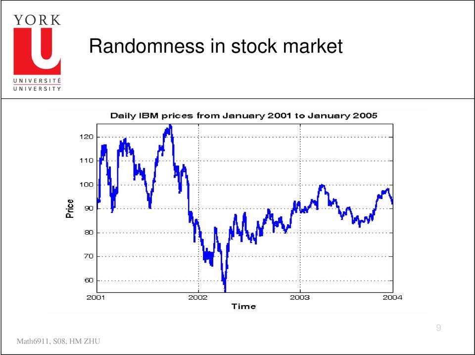
9 Randomness in stock market 9
10 Outlines 1. Markov process. Wiener process 3. Generalized Wiener process 4. Ito s process, Ito s lemma 5. Asset price models 10

11 References 1. Chapter 1, Options, Futures, and Other Derivatives. Appendix A for Introduction to MATLAB, Appendix B for review of probability theory, Numerical Methods in Finance: A MATLAB Introduction 11

12 Markov process A particular type of stochastic process whose future probability depends only on the present value A stochastic process x(t) is called a Markov process if for every n and P The Markov property implies that the probability distribution of the price at any particular future time is not dependent on the particular path followed by the price in the past 1 <, we have ( x( t ) x x( t) for all t t ) = P x( t ) x x( t ) n t n t < < t n n 1 ( ) n n n 1 1
 x x( t) for all t t ) = P x( t ) x x( t ) n t n t < < t n n")
13 Modeling of asset prices Really about modeling the arrival of new info that affects the price. Under the assumptions, The past history is fully reflected in the present asset price, which does not hold any further information Markets respond immediately to any new information about an asset The anticipated changes in the asset price are a Markov process 13

14 Weak-Form Market Efficiency This asserts that it is impossible to produce consistently superior returns with a trading rule based on the past history of stock prices. In other words technical analysis does not work. A Markov process for stock prices is clearly consistent with weak-form market efficiency

15 Example of a Discrete Time Continuous Variable Model A stock price is currently at $40. Over one year, the change in stock price has a distribution Ν(0,10) where Ν(µ,σ) is a normal distribution with mean µ and standard deviation σ.
 where Ν(µ,σ) is a normal")
16 Questions What is the probability distribution of the change of the stock price over years? ½ years? ¼ years? t years? Taking limits we have defined a continuous variable, continuous time process

17 Variances & Standard Deviations In Markov processes, changes of the variable in successive periods of time are independent. This means that: Means are additive variances are additive Standard deviations are not additive

18 Variances & Standard Deviations (continued) In our example it is correct to say that the variance is 100 per year. It is strictly speaking not correct to say that the standard deviation is 10 per year.

19 A Wiener Process (See pages 65-67, Hull) Consider a variable z follows a particular Markov process with a mean change of 0 and a variance rate of 1.0 per year. The change in a small interval of time t is z The variable follows a Wiener process if 1. z = ε t where ε is N(0,1). The values of z for any different (nonoverlapping) periods of time are independent
.")
20 Properties of a Wiener Process z over a small time interval t: Mean of z is 0 Variance of z is t Standard deviation of z is t z over a long period of time, T: Mean of [z (T ) z (0)] is 0 Variance of [z (T ) z (0)] is T Standard deviation of [z (T ) z (0)] is T
![over a long period of time, T: Mean of [z (T ) z (0)] is 0](/docs-images/43/19194241/images/page_20.jpg "Variance of [z (T ) z (0)] is T Standard deviation of [z (T ) z")
21 Taking Limits... What does an expression involving dz and dt mean? It should be interpreted as meaning that the corresponding expression involving z and t is true in the limit as t tends to zero In this respect, stochastic calculus is analogous to ordinary calculus
22 Generalized Wiener Processes (See page 67-69, Hull) A Wiener process has a drift rate (i.e. average change per unit time) of 0 and a variance rate of 1 In a generalized Wiener process the drift rate and the variance rate can be set equal to any chosen constants The variable x follows a generalized Wiener process with a drift rate of a and a variance rate of b if dx=a dt + b dz
23 Generalized Wiener Processes (continued) x = a t + b ε t Mean change in x in time t is a t Variance of change in x in time t is b t Standard deviation of change in x in time t is b t
24 Generalized Wiener Processes (continued) Mean change in x in time T is at Variance of change in x in time T is b T Standard deviation of change in x in time T is b T x= a T+ b ε T
25 Example A stock price starts at 40 and at the end of one year, it has a probability distribution of N(40,10) If we assume the stochastic process is Markov with no drift then the process is ds = 10dz If the stock price were expected to grow by $8 on average during the year, so that the year-end distribution is N (48,10), the process would be ds = 8dt + 10dz What the probability distribution of the stock price at the end of six months?
26 Itô Process (See pages 69, Hull) In an Itô process the drift rate and the variance rate are functions of time dx=a(x,t) dt+b(x,t) dz The discrete time version, i.e., x over a small time interval (t, t+ t) x = a( x, t) t + b( x, t) ε t is only true in the limit as t tends to zero
27 Why a Generalized Wiener Process is not Appropriate for Stocks For a stock price we can conjecture that its expected percentage change in a short period of time remains constant, not its expected absolute change in a short period of time We can also conjecture that our uncertainty as to the size of future stock price movements is proportional to the level of the stock price
28 A Simple Model for Stock Prices (See pages 69-71, Hull) ds = µ S dt + σ S dz Itô s process where µ is the expected return σ is the volatility. The discrete time equivalent is S = µ S t + σsε t
29 Example: Simulate asset prices Consider a stock that pays no-dividends, has an expected return 15% per annum with continuous compounding and a volatility of 30% per annum. Observe today s price $1 per share and with t = 1/50 yr. Simulate a path for the stock price. Given Then S i -1 i, we compute S = µ S t + σs ε t i 1 i 1 S = S + S i 1 9
30 Example: Simulate stock prices Stock Price S at start of period Random sample for ε S during a time period dt
31 Example: Simulate stock prices 31
32 Itô s Lemma (See pages 73-74, Hull) If we know the stochastic process followed by x, Itô s lemma tells us the stochastic process followed by some function G (x, t ) Since a derivative security is a function of the price of the underlying and time, Itô s lemma plays an important part in the analysis of derivative securities
33 Taylor Series Expansion A Taylor s series expansion of G(x, t) gives = t t G t x t x G x x G t t G x x G G ½ ½
34 Ignoring Terms of Higher Order Than t and x t x x x G t t G x x G G t t G x x G G + + = + = ½ order of which is has a component because In stochastic calculus this becomes In ordinary calculus we have
35 Substituting for x t b x G t t G x x G G t t b t a x dz t x b dt t x a dx ε + + = ε + = ½ higher order than Then ignoring terms of + = so that ), ( ), ( Suppose
36 The ε t Term Since ε N(0,1), E( ε ) = 0 It follows that ( ε ) ( ε ) [ ( ε)] = 1 ( ε ) = 1 The variance of is proportional to and can be ignored. Hence G G 1 G G x t b t = + + x t x E E E t = t t E t
37 Taking Limits s Lemma is Ito' This ½ obtain We ng Substituti ½ limits Taking dz b x G dt b x G t G a x G dg dz b dt a dx dt b x G dt t G dx x G dg = + = + + =
38 Application of Ito s Lemma to a Stock Price Process The stock price process is ds = µ S dt + σs d z For a function G of S and t dg = G S µ S + G t + ½ G S σ S dt + G S σs dz
39 Example If G = ln S, then dg =? σ dg = µ dt + σ dz Generalized Wiener process
40 A generalized Wiener process for stock price The discrete version of this is or () t ( /) St ( + t) = St ( ) e ( ) ln St ( + t) ln St ( ) = µ σ / t+ σε t µ σ t+ σ ε t S follows a lognormal distribution. It is often referred to as geometric Brownian motion. 40
41 Lognormal Distribution The corresponding density function for S( t) is ( x) f exp = ( ()) ( ) for x > 0 with f x = 0 for x 0. It can be proven that E S t = S e var ( ()) ( µ + σ ) = 0 ( ()) 0 µ t E S t S e log x σ µ t S 0 σ t xσ πt µ t σ = ( t ) 0 1 S t S e e t
42 Example: Simulate stock prices 4
43 Models for stock price in risk neutral world (r: risk-free interest rate) In a risk neutral world, two process for the underlying asset is: ds = σ S dz + ˆ µ Sdt or (1) ( ) () ˆ () () S t + t S t = µ S t t + σs t ε t ( σ ) d ln S= r / dt+ σ dz or () ( σ ) ln St ( + t) ln St ( ) = r / t+ σε t 43
44 Which one is more accurate? It is usually more accurate to work with InS because it follows a generalized Wiener process and () is true for any t while (1) is true only in the limit as t tends to zero. For all T, ( σ ) ln ST ( ) ln S(0) = r / T + σε T i.e., ( r /) T ST ( ) S(0) e σ + = σε T 44
45 3. Monte Carlo Simulation 3.3 Generate pseudo-random variates Math6911 S08, HM Zhu
46 Generate pseudorandom variates The usual way to generate psedorandom variates, i.e., samples from a given probability distribution: 1. Generate psedurandom numbers, which are variates from the uniform distribution on the interval (0, 1). Denote as U(0, 1). Apply suitable transformation to obtain the desired distribution
47 Generate U(0, 1) variables The standard method is linear congruential generators (LCGs): 1.. Return number Comments : Z Given an integer number Z ( az + c)( mod m) where a, c, and m are chosen parameters 0 Z i = i 1 Zi m : the initial number, the seed of which generate a U(0,1) variable eg. rand('seed', 0) generates the same sequence each time LCGs generates rational numbers instead of i-1, the random sequence. m-1 real ones i Periodic. The sequency Ui = has a maximum period of m m i= 0 Improved MATLAB function :rand('state', 0) allows much longer periods
48 Generate U(0, 1) variables
49 Generate U(0, 1) variables
50 Generate general distribution F(x) from U(0, 1) Given the distribution function F. Return X = F -1 ( U ) ( x) = P{ X x} random variates according to F by the following 1. Draw a random number U~U ( 01, ), we can generate Proof : Use the monotonicity of F and the fact that U is distributed : P 1 { X x} = P F ( U ) { } = F( x) { x} = P U F( x) uniformly
51 Question How to generate samples according to standard normal distribution N(0,1) from U(0, 1)? - No analytical form of the inverse of the distribution function - Support is not finite
52 Generate Samples from Normal Distribution One simple way to obtain a sample from Ν(0,1) is as follows where U and x is i 1 x = i= 1 U i 6 ( ) the required samples from N 0,1 ( ) are independent random numbers from U 0,1, Note : - It is from Central Limit Theorem. - The approximation is satisfactory for most purposes
53 Central Limit Theorem Let X 1, X, X 3,... be a sequence of independent random variables which has the same probability distribution. Consider the sum :S n = X X n. Then the expected value of S n is nμ and its standard deviation is σ n ½. Furthermore, informally speaking, the distribution of S n approaches the normal distribution N(nμ,σn 1/ ) as n approaches. Or the standardized S n, i.e., Then the distribution of Z n converges towards the standard normal distribution N(0,1) as n approaches
54 A Note Uniform random variable X: PDF: 1, if x a,b f ( x) = b a 0, otherwise Mean: b+ a EX [ ] = Variance: Var ( X ) = ( b a) 1 ( )
55 Generate Samples from N(0,1): Box-Muller algorithm The Box-Muller algorithm can be implemented as follows:. Set R logu1 and = U 1 ( ) 1. Generate two independent uniform samples from U,U ~ U 0, 1 = 3. Set X = Rcosθ and Y = Rsinθ θ where X and Y are independent samples from N 0, 1. π ( ) Note: - Box and Muller (1958), Ann. Math. Statist., 9: Common and more efficient than the previous method. - But it is costly to evaluate trigonometric functions
56 Generate Samples from N(0,1): Improved Box-Muller algorithm The polar rejection (improved Box-Muller) method: ( ) 1. Generate two independent uniform samples from U,U ~ U 0, 1. Set V = U -1, V = U -1, and S = V + V 3. If S>1, return to step 1; otherwise, return -lns -lns X = V and Y = V S S 1 ( ) where X and Y are required independent samples from N 0, 1. Note: - Ahrens and Dieter (1988), Comm. ACM 31:
57 Question How to generate samples according to normal distribution N(µ, σ) from N(0, 1)?
58 To Obtain Correlated Normal Samples To obtain correlated normal samples ε and ε, we first generate two independent stardard normal variates x, x ~N 0,1. and set ε = µ + x ε = µ + ρx + x 1 ρ where ρ is the coefficient of correlation. 1 ( )
59 To Obtain n Correlated Normal Samples To obtain n correlated normal samples ε,, ε, we first 1. generate n independent stardard normal variates x,,x ~N 0,1. and set T ε µ U X = n T Here, UU= Σ = ρ ij is the Cholesky decomposition of the covariance matrix Σ. n ( )
60 Simulate the correlated asset prices To simulate the payoff of a derivative depending on multi-variables, how can we generate samples of each variables? ( ) S(t+ t) = S(t)e µ i σi σiεi i i ˆ / + t t 60
61 3. Monte Carlo Simulation 3.4 Choose the number of simulations Math6911 S08, HM Zhu
62 How many trials is enough? X i : Sequence of independent samples from the same distribution ( ) X M 1 M M i=1 ( ) = ( ) S M 1 Xi X M M 1 X i M i=1 : Sample mean, an unbiased estimator to the [ ] quantitiy of interest µ = E X : Sample variance E σ ( ( ) µ ) X M = Var X ( M) = : the expected value of square error M as a way to quantify the quality of our estimator Note that can be estimated by the sample vari σ i ance S ( M)
63 Number of Simulations and Accuracy The number of simulation trials carried out depends on the accuracy required. M: number of independent trials carried out µ: expected value of the derivative, S(M): standard deviation of the discounted payoff given by the trials.
64 Standard Errors in Monte Carlo Simulation The standard error of the estimate of the option price based on sample size M is: σ M S ( M) M Clearly as M increases, our estimate is more accurate
65 (1-α) Confidence Interval of Monte Carlo Simulation In general, the confident interval at level (1- α) may be computed by 1 α / ( ) S M S M ( ) 1 α / µ 1 α / Note: Uncertainty is inverse proportional to the square root of the number of trials ( ) X ( M) z < < X M + z M M where z is the critical number from the standard normal distribution.
66 95% Confidence Interval of Monte Carlo Simulation A 95% confidence interval for the price V of the derivative is therefore given by: ( ) X M ( ) ( ) ( ) S M S M 1.96 < µ < X M M M
67 Absolute error Suppose we want to controlling the absolute error such that, with probability 1-α, ( ) ( ) X M µ β, where β is the maximum acceptable tolerance. Then the number of simulations M must satisfy β z ( ) 1 α / S M M.
68 Relative error Suppose we want to controlling the relative error such that, with probability 1-α, X M ( ) µ ( ) ( ) µ γ, where γ is the maximum acceptable tolerance. Then the number of simulations M must satisfy z ( ) 1 α / S M M X M 1. γ + γ
69 3. Monte Carlo Simulation 3.5 Applications in Option Pricing Math6911 S08, HM Zhu
70 Monte Carlo Simulation When used to value a derivative dependent on a market variable S, this involves the following steps: 1. Simulate 1 path for the stock price in a risk-neutral world. Calculate the payoff from the stock option 3. Repeat steps 1 and many times to get many sample payoff 4. Calculate mean payoff 5. Discount mean payoff at risk-free rate to get an estimate of the value of the option
71 Example: European call Consider a European call on a stock with no-dividend payment. S(0) = $50, E = 5, T = 5 months, and annual risk-free interest rate r = 10% and a volatility σ= 40% per annum. Black-Schole Price: $ MC Price with 1000 simulations: $ Confidence Interval [4.8776, ] MC Price with 00,000 simulations: $ Confidence Interval [5.1393, 5.167] 71
72 Example: Butterfly Spread A butterfly spread consists of buying a European call option with exercise price K 1 and another with exercise price K 3 (K 1 < K 3 ) and by selling two calls with exercise price K = (K 1 + K 3 )/, for the same asset and expiry date Consider a butterfly spread with S(0) = $50, K 1 = $55, K = $60, K 3 = 65, T = 5 months, and annual risk-free interest rate r = 10% and a volatility σ= 40% per annum. Exact price: $0.614 MC price with 100,000 simulations: $ Confidence Interval [0.6017, ] 7
73 Example: Arithmetic Average Asian Option Consider pricing an Asian average rate call option with discrete arithmetic averaging. The option payoff is 1 N max S ( ti ) K, 0 N i= 1 where ti = i t and = t T. N Consider the option on a stock with no-dividend payment. S(0) = $50, K = 50, T = 5 months, and annual risk-free interest rate r = 10% and a volatility σ= 40% per annum. 73
74 Determining Greek Letters For : 1. Make a small change to asset price. Carry out the simulation again using the same random number streams 3. Estimate as the change in the option price divided by the change in the asset price V * MC V S MC Proceed in a similar manner for other Greek letters 74
75 3. Monte Carlo Simulation 3.6 Further Comments Math6911 S08, HM Zhu
76 The parameters in the model Our analysis so far is useless unless we know the parameters µ and σ The price of an option or derivative is in general independent of µ However, the asset price volatility σ is critically important to option price. Typically, 0%< σ < 50% Volatility of stock price can be defined as the standard deviation of the return provided by the stock in one year when the return is expressed using continuous compounding 76
77 Estimate volatility σ from historical data Assume: n + 1: number of observation at fixed time interval S: i Stock price at end of ith (i = 0, 1,..., n) interval t: Length of observing time interval in years S i ui = ln : n number of approximation for the change Si 1 of ln S over t 77
78 Estimate volatility σ from historical data Compute the standard deviation of the u 1 n ( ) s = u 1 i u i= n 1 where the mean of the u 'sis s The standard error of estimate is about 1 n u = u i= 1 i n s σ t σ ˆ σ = t i i 's: ˆ σ n 78
79 Advantages and Limitations More efficient for options dependent on multiple underlying stochastic variables. As the number of variables increase, Monte Carlo simulations increases linearly while the others increases exponentially Easily deal with path dependent options and options with complex payoffs / complex stochastic processes Has an error estimate It cannot easily deal with American options Very time-consuming
80 Extensions to multiple variables When a derivative depends on several underlying variables we can simulate paths for each of them in a risk-neutral world to calculate the values for the derivative
81 Sampling Through the Tree Instead of sampling from the stochastic process we can sample paths randomly through a binomial or trinomial tree to value a derivative
82 3. Monte Carlo Simulation 3.7 Variance Reduction Techniques Math6911 S08, HM Zhu
83 Variance Reduction Procedures Usually, a very large value of M is needed to estimate V with reasonable accuracy. Variance reduction techniques lead to dramatic savings in computational time Antithetic variable technique Control variate technique Importance sampling Stratified sampling Moment matching Using quasi-random sequences
84 Antithetic Variable Technique 1 VAV = M We can prove that ( ( )) ( 01) Consider to estimate V = E f U where U N,. The standard Monte Carlo estimate: M 1 V = f U U N,. ( ) with i.i.d. ( 01) MC i i M i= 1 The antithetic variate technique: M i= 1 ( ) + ( ) ( i) + ( i) with i.i.d. U N ( 01, ) f U f U f Ui f Ui 1 var = var ( f ( Ui) ) cov( f ( U i), f ( Ui) ) + 1 var ( f ( Ui )) if f is monotonic. i
85 Antithetic Variable Technique It involves calculating two values of the derivative. V 1 : calculated in the usual way V : calculated by the changing the sign of all the random standard normal samples used for V 1 V is average of the V 1 and V, the final estimate of the value of the derivative
86 Antithetic Variable Technique Note: 1. Monte-Carlo works when the simulated variables "spread out" as closely as possible to the true distribution.. Antithetic variates relies upon finding samplings that are anticorrelated with the original random variable. 3. Works well when the payoff is monotonic w.r.t. S 4. Further reading: --P.P. Boyle, Option: a Monte Carlo approach, J. of Finanical Economics, 4: (1977) --Boyle, Broadie and Glasserman, Monte Carlo methods for security pricing J. of Economic Dynamics and Control, 1: (1997) --N. Madras, Lectures on Monte Carlo Methods, 00
87 Example: European call Consider a European call on a stock with no-dividend payment. S(0) = $50, K = 5, T = 5 months, and annual risk-free interest rate r = 10% and a volatility σ= 40% per annum. Black-Schole Price: $ MC Price with 00,000 simulations: $ Confidence Interval [5.1393, 5.167] MCAV Price with 00,000 simulations: $ Confidence Interval [5.1615, 5.058] (ratio: 1.75) 87
88 Example: Butterfly Spread Consider a butterfly spread with S(0) = $50, K 1 = $55, K = $60, K 3 = 65, T = 5 months, and annual risk-free interest rate r = 10% and a volatility σ= 40% per annum. Exact price: $0.614 MC price with 100,000 simulations: $ Confidence Interval [0.6017, ] MCAV price with 50,000 simulations: $ Confidence Interval [0.598, ] 88
89 Control Variate Technique We can generalize the previous technique to ( ( ) ) for any θ. Here, V is "close" to V with known mean E V. In this case, Z = V + θ E V V θ var A B B Z = var V θv ( ) ( ) θ ( ) B A B A B = var V θcov V, V + θ var V ( ) ( ) ( ) We can prove that var Z < var V if and only if cov VA, V 0< θ < var V A A B B ( ) ( ) θ ( ) ( ) B B. A 89
90 Example: European call Consider a European call on a stock with no-dividend payment. S(0) = $50, K = 5, T = 5 months, and annual risk-free interest rate r = 10% and a volatility σ= 40% per annum. Black-Schole Price: $ MC Price with 00,000 simulations: $ Confidence Interval [5.1393, 5.167] MCCV Price with 00,000 simulations: $ Confidence Interval [5.171, 5.054] (ratio:.645) 90
91 Example: Arithmetic Average Asian Option Consider the option on a stock with no-dividend payment. S(0) = $50, K = 50, T = 5 months, and annual risk-free interest rate r = 10% and a volatility σ= 40% per annum. We could use the sum of the asset prices as a control variate as we know its expected value and Y is correlated to the option itself N N N r( N+ 1) t ri t 1 e E S( ti ) = E S( i t) = S0 e = S0 r t i= 0 i= 0 i= 0 1 e Another choice of the control variate is the payoff of a geometric average option as this is known analytically 1 N N max S( ti ) K, 0 i= 1 91
92 Importance Sampling Technique It is a way to distort the probability measure in order to sample from critical region. For example, in evaluating European call option: F: the unconditional probability distribution function for the asset price at time T q: the probability of the asset price K at maturity, known analytically G = F / q: the probability distribution of the asset conditional on the asset price K, i.e., importance function Instead of sampling from F, we sample from G. Then the value of the option is the average discounted payoff multiplied by q.
93 Stratified Sampling Technique Sampling representative values rather than random values from a probability distribution is usually more accurate. It involves dividing the distribution into intervals and sampling from each interval (stratum) according to the distribution: [ ] EX m = pe j XY= j= 1 { } j where P Y = y = p for j = 1,,m, is known. j y j Note: 1. For each stratum, we sample X conditioned on the even Y = y j. The representative values are typically mean or median for each interval
94 Moment Matching Moment matching involves adjusting the samples taken from a standard normal distribution so that the first, second, or possibly higher moments are matched. For example, we want to sample from N(0,1). Suppose that the samples are εi (1 i n). To match the first two moments, we adjustify the samples by * εi m εi = s where m and s are the mean and standard deviation of samples. The adjusted samples ε has the correct mean 0 and standard deviation 1. * i We then use the adjusted samples for calculation.
95 Quasi-Random Sequences Also called a low-discrepancy sequence is a sequence of representative samples from a probability distribution At each stage of the simulation, the sampled points are roughly evenly distributed throughout the probability space The standard error of the estimate is proportional to 1 M
96 Further reading R. Brotherton-Ratcliffe, Monte Carlo Motoring, Risk, 1994: W.H.Press, et al, Numerical Reciptes in C, Cambridge Univ. Press, 199 I. M. Sobol, USSR Computational Mathematics and Mathematical Physics, 7, 4, (1967): 86-11; P. Jaeckel, Monte Carlo Methods in finance, Wiley, Chichester, 00 P. Glasserman, Monte Carlo Methods in Financial Engineering, Springer-Verlag, New York, 004
97 Further reading
98 3. Monte Carlo Simulation Appendix Math6911 S08, HM Zhu
99 Asian Options (Chapter ) Payoff related to average stock price Average Price options pay: Call: max(s ave K, 0) Put: max(k S ave, 0) Average Strike options pay: Call: max(s T S ave, 0) Put: max(s ave S T, 0) 99
100 Asian Options (Chapter ) For arithmetic averaging: N 1 S S t, T N t ave For geometric averaging: = ( ) i where = N i = 1 S N ave = S t1 S t S tn ( ) ( ) ( ) 10 0
101 Asian Options (geometric averaging) Closed form (Kemna & Vorst,1990, J. of Banking and Finance, 14:113-19) because the geometric average of the underlying prices follows a lognormal distribution as well. where N(x) is the cumulative normal distribution function and 10 1
102 Asian Options (arithmetic averaging) No analytic solution Can be valued by assuming (as an approximation) that the average stock price is lognormally distributed Turnbull and Wakeman, 1991, J. of Financial and Quantitative Finance, 6: Levy,199, J. of International Money and Finance, 14:
103 Example: Asian Put with arithmetric average Consider an Asian Put on a stock with non-dividend payment. S(0) = $50, X = 50, T = 5 months, and annual risk-free interest rate r = 10% and a volatility σ= 40% per annum. MC Price with 100,000 simulations: $ Confidence Interval [3.9195, 4.07] MCAV Price with 100,000 simulations: $ Confidence Interval [3.9854, ] 10 3
Generating Random Numbers Variance Reduction Quasi-Monte Carlo. Simulation Methods. Leonid Kogan. MIT, Sloan. 15.450, Fall 2010
 Simulation Methods Leonid Kogan MIT, Sloan 15.450, Fall 2010 c Leonid Kogan ( MIT, Sloan ) Simulation Methods 15.450, Fall 2010 1 / 35 Outline 1 Generating Random Numbers 2 Variance Reduction 3 Quasi-Monte
Monte Carlo Methods in Finance
 Author: Yiyang Yang Advisor: Pr. Xiaolin Li, Pr. Zari Rachev Department of Applied Mathematics and Statistics State University of New York at Stony Brook October 2, 2012 Outline Introduction 1 Introduction
Overview of Monte Carlo Simulation, Probability Review and Introduction to Matlab
 Monte Carlo Simulation: IEOR E4703 Fall 2004 c 2004 by Martin Haugh Overview of Monte Carlo Simulation, Probability Review and Introduction to Matlab 1 Overview of Monte Carlo Simulation 1.1 Why use simulation?
第 9 讲 : 股 票 期 权 定 价 : B-S 模 型 Valuing Stock Options: The Black-Scholes Model
 1 第 9 讲 : 股 票 期 权 定 价 : B-S 模 型 Valuing Stock Options: The Black-Scholes Model Outline 有 关 股 价 的 假 设 The B-S Model 隐 性 波 动 性 Implied Volatility 红 利 与 期 权 定 价 Dividends and Option Pricing 美 式 期 权 定 价 American
Numerical Methods for Option Pricing
 Chapter 9 Numerical Methods for Option Pricing Equation (8.26) provides a way to evaluate option prices. For some simple options, such as the European call and put options, one can integrate (8.26) directly
Chapter 2: Binomial Methods and the Black-Scholes Formula
 Chapter 2: Binomial Methods and the Black-Scholes Formula 2.1 Binomial Trees We consider a financial market consisting of a bond B t = B(t), a stock S t = S(t), and a call-option C t = C(t), where the
Binomial lattice model for stock prices
 Copyright c 2007 by Karl Sigman Binomial lattice model for stock prices Here we model the price of a stock in discrete time by a Markov chain of the recursive form S n+ S n Y n+, n 0, where the {Y i }
Valuing Stock Options: The Black-Scholes-Merton Model. Chapter 13
 Valuing Stock Options: The Black-Scholes-Merton Model Chapter 13 Fundamentals of Futures and Options Markets, 8th Ed, Ch 13, Copyright John C. Hull 2013 1 The Black-Scholes-Merton Random Walk Assumption
Variance Reduction. Pricing American Options. Monte Carlo Option Pricing. Delta and Common Random Numbers
 Variance Reduction The statistical efficiency of Monte Carlo simulation can be measured by the variance of its output If this variance can be lowered without changing the expected value, fewer replications
Exam MFE Spring 2007 FINAL ANSWER KEY 1 B 2 A 3 C 4 E 5 D 6 C 7 E 8 C 9 A 10 B 11 D 12 A 13 E 14 E 15 C 16 D 17 B 18 A 19 D
 Exam MFE Spring 2007 FINAL ANSWER KEY Question # Answer 1 B 2 A 3 C 4 E 5 D 6 C 7 E 8 C 9 A 10 B 11 D 12 A 13 E 14 E 15 C 16 D 17 B 18 A 19 D **BEGINNING OF EXAMINATION** ACTUARIAL MODELS FINANCIAL ECONOMICS
Jorge Cruz Lopez - Bus 316: Derivative Securities. Week 11. The Black-Scholes Model: Hull, Ch. 13.
 Week 11 The Black-Scholes Model: Hull, Ch. 13. 1 The Black-Scholes Model Objective: To show how the Black-Scholes formula is derived and how it can be used to value options. 2 The Black-Scholes Model 1.
Generating Random Variables and Stochastic Processes
 Monte Carlo Simulation: IEOR E4703 c 2010 by Martin Haugh Generating Random Variables and Stochastic Processes In these lecture notes we describe the principal methods that are used to generate random
CS 522 Computational Tools and Methods in Finance Robert Jarrow Lecture 1: Equity Options
 CS 5 Computational Tools and Methods in Finance Robert Jarrow Lecture 1: Equity Options 1. Definitions Equity. The common stock of a corporation. Traded on organized exchanges (NYSE, AMEX, NASDAQ). A common
Black-Scholes Equation for Option Pricing
 Black-Scholes Equation for Option Pricing By Ivan Karmazin, Jiacong Li 1. Introduction In early 1970s, Black, Scholes and Merton achieved a major breakthrough in pricing of European stock options and there
Generating Random Variables and Stochastic Processes
 Monte Carlo Simulation: IEOR E4703 Fall 2004 c 2004 by Martin Haugh Generating Random Variables and Stochastic Processes 1 Generating U(0,1) Random Variables The ability to generate U(0, 1) random variables
Moreover, under the risk neutral measure, it must be the case that (5) r t = µ t.
 r t = µ t.") LECTURE 7: BLACK SCHOLES THEORY 1. Introduction: The Black Scholes Model In 1973 Fisher Black and Myron Scholes ushered in the modern era of derivative securities with a seminal paper 1 on the pricing
LECTURE 7: BLACK SCHOLES THEORY 1. Introduction: The Black Scholes Model In 1973 Fisher Black and Myron Scholes ushered in the modern era of derivative securities with a seminal paper 1 on the pricing
Hedging Options In The Incomplete Market With Stochastic Volatility. Rituparna Sen Sunday, Nov 15
 Hedging Options In The Incomplete Market With Stochastic Volatility Rituparna Sen Sunday, Nov 15 1. Motivation This is a pure jump model and hence avoids the theoretical drawbacks of continuous path models.
The Black-Scholes Formula
 FIN-40008 FINANCIAL INSTRUMENTS SPRING 2008 The Black-Scholes Formula These notes examine the Black-Scholes formula for European options. The Black-Scholes formula are complex as they are based on the
The Monte Carlo Framework, Examples from Finance and Generating Correlated Random Variables
 Monte Carlo Simulation: IEOR E4703 Fall 2004 c 2004 by Martin Haugh The Monte Carlo Framework, Examples from Finance and Generating Correlated Random Variables 1 The Monte Carlo Framework Suppose we wish
Simulating Stochastic Differential Equations
 Monte Carlo Simulation: IEOR E473 Fall 24 c 24 by Martin Haugh Simulating Stochastic Differential Equations 1 Brief Review of Stochastic Calculus and Itô s Lemma Let S t be the time t price of a particular
Hedging Variable Annuity Guarantees
 p. 1/4 Hedging Variable Annuity Guarantees Actuarial Society of Hong Kong Hong Kong, July 30 Phelim P Boyle Wilfrid Laurier University Thanks to Yan Liu and Adam Kolkiewicz for useful discussions. p. 2/4
General Sampling Methods
 General Sampling Methods Reference: Glasserman, 2.2 and 2.3 Claudio Pacati academic year 2016 17 1 Inverse Transform Method Assume U U(0, 1) and let F be the cumulative distribution function of a distribution
Pricing Discrete Barrier Options
 Pricing Discrete Barrier Options Barrier options whose barrier is monitored only at discrete times are called discrete barrier options. They are more common than the continuously monitored versions. The
Stephane Crepey. Financial Modeling. A Backward Stochastic Differential Equations Perspective. 4y Springer
 Stephane Crepey Financial Modeling A Backward Stochastic Differential Equations Perspective 4y Springer Part I An Introductory Course in Stochastic Processes 1 Some Classes of Discrete-Time Stochastic
Monte Carlo Simulation
 1 Monte Carlo Simulation Stefan Weber Leibniz Universität Hannover email: sweber@stochastik.uni-hannover.de web: www.stochastik.uni-hannover.de/ sweber Monte Carlo Simulation 2 Quantifying and Hedging
OPTION PRICING FOR WEIGHTED AVERAGE OF ASSET PRICES
 OPTION PRICING FOR WEIGHTED AVERAGE OF ASSET PRICES Hiroshi Inoue 1, Masatoshi Miyake 2, Satoru Takahashi 1 1 School of Management, T okyo University of Science, Kuki-shi Saitama 346-8512, Japan 2 Department
Lecture 12: The Black-Scholes Model Steven Skiena. http://www.cs.sunysb.edu/ skiena
 Lecture 12: The Black-Scholes Model Steven Skiena Department of Computer Science State University of New York Stony Brook, NY 11794 4400 http://www.cs.sunysb.edu/ skiena The Black-Scholes-Merton Model
An Introduction to Modeling Stock Price Returns With a View Towards Option Pricing
 An Introduction to Modeling Stock Price Returns With a View Towards Option Pricing Kyle Chauvin August 21, 2006 This work is the product of a summer research project at the University of Kansas, conducted
1 The Black-Scholes model: extensions and hedging
 1 The Black-Scholes model: extensions and hedging 1.1 Dividends Since we are now in a continuous time framework the dividend paid out at time t (or t ) is given by dd t = D t D t, where as before D denotes
The Black-Scholes pricing formulas
 The Black-Scholes pricing formulas Moty Katzman September 19, 2014 The Black-Scholes differential equation Aim: Find a formula for the price of European options on stock. Lemma 6.1: Assume that a stock
14 Greeks Letters and Hedging
 ECG590I Asset Pricing. Lecture 14: Greeks Letters and Hedging 1 14 Greeks Letters and Hedging 14.1 Illustration We consider the following example through out this section. A financial institution sold
Review of Basic Options Concepts and Terminology
 Review of Basic Options Concepts and Terminology March 24, 2005 1 Introduction The purchase of an options contract gives the buyer the right to buy call options contract or sell put options contract some
INTEREST RATES AND FX MODELS
 INTEREST RATES AND FX MODELS 8. Portfolio greeks Andrew Lesniewski Courant Institute of Mathematical Sciences New York University New York March 27, 2013 2 Interest Rates & FX Models Contents 1 Introduction
On Black-Scholes Equation, Black- Scholes Formula and Binary Option Price
 On Black-Scholes Equation, Black- Scholes Formula and Binary Option Price Abstract: Chi Gao 12/15/2013 I. Black-Scholes Equation is derived using two methods: (1) risk-neutral measure; (2) - hedge. II.
Basics of Statistical Machine Learning
 CS761 Spring 2013 Advanced Machine Learning Basics of Statistical Machine Learning Lecturer: Xiaojin Zhu jerryzhu@cs.wisc.edu Modern machine learning is rooted in statistics. You will find many familiar
Quantitative Methods for Finance
 Quantitative Methods for Finance Module 1: The Time Value of Money 1 Learning how to interpret interest rates as required rates of return, discount rates, or opportunity costs. 2 Learning how to explain
The Black-Scholes-Merton Approach to Pricing Options
 he Black-Scholes-Merton Approach to Pricing Options Paul J Atzberger Comments should be sent to: atzberg@mathucsbedu Introduction In this article we shall discuss the Black-Scholes-Merton approach to determining
Pricing Barrier Option Using Finite Difference Method and MonteCarlo Simulation
 Pricing Barrier Option Using Finite Difference Method and MonteCarlo Simulation Yoon W. Kwon CIMS 1, Math. Finance Suzanne A. Lewis CIMS, Math. Finance May 9, 000 1 Courant Institue of Mathematical Science,
Hedging Illiquid FX Options: An Empirical Analysis of Alternative Hedging Strategies
 Hedging Illiquid FX Options: An Empirical Analysis of Alternative Hedging Strategies Drazen Pesjak Supervised by A.A. Tsvetkov 1, D. Posthuma 2 and S.A. Borovkova 3 MSc. Thesis Finance HONOURS TRACK Quantitative
Mathematical Finance
 Mathematical Finance Option Pricing under the Risk-Neutral Measure Cory Barnes Department of Mathematics University of Washington June 11, 2013 Outline 1 Probability Background 2 Black Scholes for European
1 Sufficient statistics
 1 Sufficient statistics A statistic is a function T = rx 1, X 2,, X n of the random sample X 1, X 2,, X n. Examples are X n = 1 n s 2 = = X i, 1 n 1 the sample mean X i X n 2, the sample variance T 1 =
Option Pricing Methods for Estimating Capacity Shortages
 Option Pricing Methods for Estimating Capacity Shortages Dohyun Pak and Sarah M. Ryan Department of Industrial and Manufacturing Systems Engineering Iowa State University Ames, IA 500-64, USA Abstract
LogNormal stock-price models in Exams MFE/3 and C/4
 Making sense of... LogNormal stock-price models in Exams MFE/3 and C/4 James W. Daniel Austin Actuarial Seminars http://www.actuarialseminars.com June 26, 2008 c Copyright 2007 by James W. Daniel; reproduction
Valuation of Asian Options
 Valuation of Asian Options - with Levy Approximation Master thesis in Economics Jan 2014 Author: Aleksandra Mraovic, Qian Zhang Supervisor: Frederik Lundtofte Department of Economics Abstract Asian options
Monte Carlo simulation techniques
 Monte Carlo simulation techniques -The development of a general framework Master s Thesis carried out at the Department of Management and Engineering, Linköping Institute of Technology and at Algorithmica
Maximum Likelihood Estimation
 Math 541: Statistical Theory II Lecturer: Songfeng Zheng Maximum Likelihood Estimation 1 Maximum Likelihood Estimation Maximum likelihood is a relatively simple method of constructing an estimator for
1 The Brownian bridge construction
 The Brownian bridge construction The Brownian bridge construction is a way to build a Brownian motion path by successively adding finer scale detail. This construction leads to a relatively easy proof
S 1 S 2. Options and Other Derivatives
 Options and Other Derivatives The One-Period Model The previous chapter introduced the following two methods: Replicate the option payoffs with known securities, and calculate the price of the replicating
Monte Carlo Simulation
 Lecture 4 Monte Carlo Simulation Lecture Notes by Jan Palczewski with additions by Andrzej Palczewski Computational Finance p. 1 We know from Discrete Time Finance that one can compute a fair price for
TABLE OF CONTENTS. A. Put-Call Parity 1 B. Comparing Options with Respect to Style, Maturity, and Strike 13
 TABLE OF CONTENTS 1. McDonald 9: "Parity and Other Option Relationships" A. Put-Call Parity 1 B. Comparing Options with Respect to Style, Maturity, and Strike 13 2. McDonald 10: "Binomial Option Pricing:
Vanna-Volga Method for Foreign Exchange Implied Volatility Smile. Copyright Changwei Xiong 2011. January 2011. last update: Nov 27, 2013
 Vanna-Volga Method for Foreign Exchange Implied Volatility Smile Copyright Changwei Xiong 011 January 011 last update: Nov 7, 01 TABLE OF CONTENTS TABLE OF CONTENTS...1 1. Trading Strategies of Vanilla
Credit Risk Models: An Overview
 Credit Risk Models: An Overview Paul Embrechts, Rüdiger Frey, Alexander McNeil ETH Zürich c 2003 (Embrechts, Frey, McNeil) A. Multivariate Models for Portfolio Credit Risk 1. Modelling Dependent Defaults:
HPCFinance: New Thinking in Finance. Calculating Variable Annuity Liability Greeks Using Monte Carlo Simulation
 HPCFinance: New Thinking in Finance Calculating Variable Annuity Liability Greeks Using Monte Carlo Simulation Dr. Mark Cathcart, Standard Life February 14, 2014 0 / 58 Outline Outline of Presentation
Efficiency and the Cramér-Rao Inequality
 Chapter Efficiency and the Cramér-Rao Inequality Clearly we would like an unbiased estimator ˆφ (X of φ (θ to produce, in the long run, estimates which are fairly concentrated i.e. have high precision.
The Heston Model. Hui Gong, UCL http://www.homepages.ucl.ac.uk/ ucahgon/ May 6, 2014
 Hui Gong, UCL http://www.homepages.ucl.ac.uk/ ucahgon/ May 6, 2014 Generalized SV models Vanilla Call Option via Heston Itô s lemma for variance process Euler-Maruyama scheme Implement in Excel&VBA 1.
Lecture 6: Option Pricing Using a One-step Binomial Tree. Friday, September 14, 12
 Lecture 6: Option Pricing Using a One-step Binomial Tree An over-simplified model with surprisingly general extensions a single time step from 0 to T two types of traded securities: stock S and a bond
Probability Generating Functions
 page 39 Chapter 3 Probability Generating Functions 3 Preamble: Generating Functions Generating functions are widely used in mathematics, and play an important role in probability theory Consider a sequence
Department of Mathematics, Indian Institute of Technology, Kharagpur Assignment 2-3, Probability and Statistics, March 2015. Due:-March 25, 2015.
 Department of Mathematics, Indian Institute of Technology, Kharagpur Assignment -3, Probability and Statistics, March 05. Due:-March 5, 05.. Show that the function 0 for x < x+ F (x) = 4 for x < for x
Alternative Price Processes for Black-Scholes: Empirical Evidence and Theory
 Alternative Price Processes for Black-Scholes: Empirical Evidence and Theory Samuel W. Malone April 19, 2002 This work is supported by NSF VIGRE grant number DMS-9983320. Page 1 of 44 1 Introduction This
Additional questions for chapter 4
 Additional questions for chapter 4 1. A stock price is currently $ 1. Over the next two six-month periods it is expected to go up by 1% or go down by 1%. The risk-free interest rate is 8% per annum with
QUANTIZED INTEREST RATE AT THE MONEY FOR AMERICAN OPTIONS
 QUANTIZED INTEREST RATE AT THE MONEY FOR AMERICAN OPTIONS L. M. Dieng ( Department of Physics, CUNY/BCC, New York, New York) Abstract: In this work, we expand the idea of Samuelson[3] and Shepp[,5,6] for
The Behavior of Bonds and Interest Rates. An Impossible Bond Pricing Model. 780 w Interest Rate Models
 780 w Interest Rate Models The Behavior of Bonds and Interest Rates Before discussing how a bond market-maker would delta-hedge, we first need to specify how bonds behave. Suppose we try to model a zero-coupon
Stock Price Dynamics, Dividends and Option Prices with Volatility Feedback
 Stock Price Dynamics, Dividends and Option Prices with Volatility Feedback Juho Kanniainen Tampere University of Technology New Thinking in Finance 12 Feb. 2014, London Based on J. Kanniainen and R. Piche,
Caput Derivatives: October 30, 2003
 Caput Derivatives: October 30, 2003 Exam + Answers Total time: 2 hours and 30 minutes. Note 1: You are allowed to use books, course notes, and a calculator. Question 1. [20 points] Consider an investor
Arbitrage-Free Pricing Models
 Arbitrage-Free Pricing Models Leonid Kogan MIT, Sloan 15.450, Fall 2010 c Leonid Kogan ( MIT, Sloan ) Arbitrage-Free Pricing Models 15.450, Fall 2010 1 / 48 Outline 1 Introduction 2 Arbitrage and SPD 3
Summary of Formulas and Concepts. Descriptive Statistics (Ch. 1-4)
") Summary of Formulas and Concepts Descriptive Statistics (Ch. 1-4) Definitions Population: The complete set of numerical information on a particular quantity in which an investigator is interested. We assume
Summary of Formulas and Concepts Descriptive Statistics (Ch. 1-4) Definitions Population: The complete set of numerical information on a particular quantity in which an investigator is interested. We assume
Chapter 3 RANDOM VARIATE GENERATION
 Chapter 3 RANDOM VARIATE GENERATION In order to do a Monte Carlo simulation either by hand or by computer, techniques must be developed for generating values of random variables having known distributions.
Does Black-Scholes framework for Option Pricing use Constant Volatilities and Interest Rates? New Solution for a New Problem
 Does Black-Scholes framework for Option Pricing use Constant Volatilities and Interest Rates? New Solution for a New Problem Gagan Deep Singh Assistant Vice President Genpact Smart Decision Services Financial
Pricing of a worst of option using a Copula method M AXIME MALGRAT
 Pricing of a worst of option using a Copula method M AXIME MALGRAT Master of Science Thesis Stockholm, Sweden 2013 Pricing of a worst of option using a Copula method MAXIME MALGRAT Degree Project in Mathematical
Understanding Options and Their Role in Hedging via the Greeks
 Understanding Options and Their Role in Hedging via the Greeks Bradley J. Wogsland Department of Physics and Astronomy, University of Tennessee, Knoxville, TN 37996-1200 Options are priced assuming that
Two Topics in Parametric Integration Applied to Stochastic Simulation in Industrial Engineering
 Two Topics in Parametric Integration Applied to Stochastic Simulation in Industrial Engineering Department of Industrial Engineering and Management Sciences Northwestern University September 15th, 2014
Lecture 1: Asset pricing and the equity premium puzzle
 Lecture 1: Asset pricing and the equity premium puzzle Simon Gilchrist Boston Univerity and NBER EC 745 Fall, 2013 Overview Some basic facts. Study the asset pricing implications of household portfolio
One Period Binomial Model
 FIN-40008 FINANCIAL INSTRUMENTS SPRING 2008 One Period Binomial Model These notes consider the one period binomial model to exactly price an option. We will consider three different methods of pricing
Chapter 13 The Black-Scholes-Merton Model
 Chapter 13 The Black-Scholes-Merton Model March 3, 009 13.1. The Black-Scholes option pricing model assumes that the probability distribution of the stock price in one year(or at any other future time)
Overview of Violations of the Basic Assumptions in the Classical Normal Linear Regression Model
 Overview of Violations of the Basic Assumptions in the Classical Normal Linear Regression Model 1 September 004 A. Introduction and assumptions The classical normal linear regression model can be written
PRICING OF GAS SWING OPTIONS. Andrea Pokorná. UNIVERZITA KARLOVA V PRAZE Fakulta sociálních věd Institut ekonomických studií
 9 PRICING OF GAS SWING OPTIONS Andrea Pokorná UNIVERZITA KARLOVA V PRAZE Fakulta sociálních věd Institut ekonomických studií 1 Introduction Contracts for the purchase and sale of natural gas providing
An introduction to Value-at-Risk Learning Curve September 2003
 An introduction to Value-at-Risk Learning Curve September 2003 Value-at-Risk The introduction of Value-at-Risk (VaR) as an accepted methodology for quantifying market risk is part of the evolution of risk
CHAPTER 6: Continuous Uniform Distribution: 6.1. Definition: The density function of the continuous random variable X on the interval [A, B] is.
![CHAPTER 6: Continuous Uniform Distribution: 6.1. Definition: The density function of the continuous random variable X on the interval [A, B] is.](/thumbs/40/21160284.jpg "CHAPTER 6: Continuous Uniform Distribution: 6.1. Definition: The density function of the continuous random variable X on the interval [A, B] is.") Some Continuous Probability Distributions CHAPTER 6: Continuous Uniform Distribution: 6. Definition: The density function of the continuous random variable X on the interval [A, B] is B A A x B f(x; A,
Some Continuous Probability Distributions CHAPTER 6: Continuous Uniform Distribution: 6. Definition: The density function of the continuous random variable X on the interval [A, B] is B A A x B f(x; A,
Monte Carlo Methods and Models in Finance and Insurance
 Chapman & Hall/CRC FINANCIAL MATHEMATICS SERIES Monte Carlo Methods and Models in Finance and Insurance Ralf Korn Elke Korn Gerald Kroisandt f r oc) CRC Press \ V^ J Taylor & Francis Croup ^^"^ Boca Raton
 A Memory Reduction Method in Pricing American Options Raymond H. Chan Yong Chen y K. M. Yeung z Abstract This paper concerns with the pricing of American options by simulation methods. In the traditional
Lectures. Sergei Fedotov. 20912 - Introduction to Financial Mathematics. No tutorials in the first week
 Lectures Sergei Fedotov 20912 - Introduction to Financial Mathematics No tutorials in the first week Sergei Fedotov (University of Manchester) 20912 2010 1 / 1 Lecture 1 1 Introduction Elementary economics
Private Equity Fund Valuation and Systematic Risk
 An Equilibrium Approach and Empirical Evidence Axel Buchner 1, Christoph Kaserer 2, Niklas Wagner 3 Santa Clara University, March 3th 29 1 Munich University of Technology 2 Munich University of Technology
Numerical methods for American options
 Lecture 9 Numerical methods for American options Lecture Notes by Andrzej Palczewski Computational Finance p. 1 American options The holder of an American option has the right to exercise it at any moment
Nonparametric adaptive age replacement with a one-cycle criterion
 Nonparametric adaptive age replacement with a one-cycle criterion P. Coolen-Schrijner, F.P.A. Coolen Department of Mathematical Sciences University of Durham, Durham, DH1 3LE, UK e-mail: Pauline.Schrijner@durham.ac.uk
2WB05 Simulation Lecture 8: Generating random variables
 2WB05 Simulation Lecture 8: Generating random variables Marko Boon http://www.win.tue.nl/courses/2wb05 January 7, 2013 Outline 2/36 1. How do we generate random variables? 2. Fitting distributions Generating
Valuing equity-based payments
 E Valuing equity-based payments Executive remuneration packages generally comprise many components. While it is relatively easy to identify how much will be paid in a base salary a fixed dollar amount
Option Pricing. 1 Introduction. Mrinal K. Ghosh
 Option Pricing Mrinal K. Ghosh 1 Introduction We first introduce the basic terminology in option pricing. Option: An option is the right, but not the obligation to buy (or sell) an asset under specified
LECTURE 15: AMERICAN OPTIONS
 LECTURE 15: AMERICAN OPTIONS 1. Introduction All of the options that we have considered thus far have been of the European variety: exercise is permitted only at the termination of the contract. These
Lecture 8. Confidence intervals and the central limit theorem
 Lecture 8. Confidence intervals and the central limit theorem Mathematical Statistics and Discrete Mathematics November 25th, 2015 1 / 15 Central limit theorem Let X 1, X 2,... X n be a random sample of
Asian Option Pricing Formula for Uncertain Financial Market
 Sun and Chen Journal of Uncertainty Analysis and Applications (215) 3:11 DOI 1.1186/s4467-15-35-7 RESEARCH Open Access Asian Option Pricing Formula for Uncertain Financial Market Jiajun Sun 1 and Xiaowei
Lecture 5: Put - Call Parity
 Lecture 5: Put - Call Parity Reading: J.C.Hull, Chapter 9 Reminder: basic assumptions 1. There are no arbitrage opportunities, i.e. no party can get a riskless profit. 2. Borrowing and lending are possible
Capital Allocation and Bank Management Based on the Quantification of Credit Risk
 Capital Allocation and Bank Management Based on the Quantification of Credit Risk Kenji Nishiguchi, Hiroshi Kawai, and Takanori Sazaki 1. THE NEED FOR QUANTIFICATION OF CREDIT RISK Liberalization and deregulation
7: The CRR Market Model
 Ben Goldys and Marek Rutkowski School of Mathematics and Statistics University of Sydney MATH3075/3975 Financial Mathematics Semester 2, 2015 Outline We will examine the following issues: 1 The Cox-Ross-Rubinstein
Simple approximations for option pricing under mean reversion and stochastic volatility
 Simple approximations for option pricing under mean reversion and stochastic volatility Christian M. Hafner Econometric Institute Report EI 2003 20 April 2003 Abstract This paper provides simple approximations
More Exotic Options. 1 Barrier Options. 2 Compound Options. 3 Gap Options
 More Exotic Options 1 Barrier Options 2 Compound Options 3 Gap Options More Exotic Options 1 Barrier Options 2 Compound Options 3 Gap Options Definition; Some types The payoff of a Barrier option is path
Research on Option Trading Strategies
 Research on Option Trading Strategies An Interactive Qualifying Project Report: Submitted to the Faculty of the WORCESTER POLYTECHNIC INSTITUTE In partial fulfillment of the requirements for the Degree
Probability and Statistics Prof. Dr. Somesh Kumar Department of Mathematics Indian Institute of Technology, Kharagpur
 Probability and Statistics Prof. Dr. Somesh Kumar Department of Mathematics Indian Institute of Technology, Kharagpur Module No. #01 Lecture No. #15 Special Distributions-VI Today, I am going to introduce
STAT 830 Convergence in Distribution
 STAT 830 Convergence in Distribution Richard Lockhart Simon Fraser University STAT 830 Fall 2011 Richard Lockhart (Simon Fraser University) STAT 830 Convergence in Distribution STAT 830 Fall 2011 1 / 31
From CFD to computational finance (and back again?)
") computational finance p. 1/21 From CFD to computational finance (and back again?) Mike Giles mike.giles@maths.ox.ac.uk Oxford University Mathematical Institute Oxford-Man Institute of Quantitative Finance
computational finance p. 1/21 From CFD to computational finance (and back again?) Mike Giles mike.giles@maths.ox.ac.uk Oxford University Mathematical Institute Oxford-Man Institute of Quantitative Finance