Bubbles and Crashes in a Behavioural Finance Model

Transcription

1 SVERIGES RIKSBANK WORKING PAPER SERIES 164 Bubbles and Crashes in a Behavioural Finance Model Paul De Grauwe and Marianna Grimaldi MAY 2004

2 WORKING PAPERS ARE OBTAINABLE FROM Sveriges Riksbank Information Riksbank SE Stockholm Fax international: Telephone international: info@riksbank.se The Working Paper series presents reports on matters in the sphere of activities of the Riksbank that are considered to be of interest to a wider public. The papers are to be regarded as reports on ongoing studies and the authors will be pleased to receive comments. The views expressed in Working Papers are solely the responsibility of the authors and should not to be interpreted as reflecting the views of the Executive Board of Sveriges Riksbank.

3 Bubbles and crashes in a behavioural finance model Paul De Grauwe University of Leuven Marianna Grimaldi Sveriges Riksbank Sveriges Riksbank Working Paper Series No. 164 May 2004 Abstract We develop a simple model of the exchange rate in which agents optimize their portfolio and use different forecasting rules. They check the profitability of these rules ex post and select the more profitable one.this model produces two kinds of equilibria, a fundamental and a bubble one. In a stochastic environment the model generates a complex dynamics in which bubbles and crashes occur at unpredictable moments. We contrast these "behavioural" bubbles with "rational" bubbles. JEL code: F31, F41, G10 Keywords: exchange rate, bounded rationality, heterogeneous agents, bubbles and crashes, complex dynamics. We are very grateful for useful comments to Volker Bohm, Yin-Wong Cheung, Hans Dewachter, Roberto Dieci, Marc Flandreau, Philip Lane, Thomas Lux, Richard Lyons, Ronald McDonald, Michael Moore, Assaf Razin, Piet Sercu, Peter Sinclair, Peter Westaway. We also benefited from comments made during seminars at the BIS, the Sveriges Riksbank, the Federal Resrve Bank of Atlanta, the University of Bonn, the University of Uppsala, and the Tinbergen Institute, Rotterdam. The views expressed in this paper are solely the responsibility of the authors and should not be interpreted as reflecting the views of the Executive Board of Sveriges Riksbank. 1

4 1 Introduction A bubble is:... a sharp rise in price of an asset or a range of assets in a continuous process, with the initial rise generating expectations of further rises and attracting new buyers-generally speculators, interested in profits from trading in the asset rather than its use as earning capacity - Kindleberger(1978). Since the publication of Kindleberger s Manias, Panics, and Crashes in 1978, a large literature has flourished on bubbles and crashes in financial markets. Two key questions have been analysed in this literature. One is whether bubbles can occur in theory; the other is whether they occur in practice. In this paper we will analyse the first question. In order to analyse the question of whether bubbles can occur in theory one has to be precise about what exactly is a bubble. With the introduction of rational expectations in economic models, a bubble was given a precise meaning. It is well-known that a rational expectations model produces infinitely many solutions for the asset price. One is the fundamental solution, and the other (in fact infinitely many) is the bubble solution. The latter is an explosive path of the asset price that increasingly deviates from the fundamental, but that continues to satisfy the no-arbitrage condition. Clearly such a definition of a bubble is not interesting in a perfect foresight environment because it means that either the bubble goes on indefinetely, or if a crash is expected at some future date, the bubble will not start (because of backward induction). This has led to the efficient market view that bubbles cannot occur. The insight provided by Blanchard and Watson (see Blanchard(1979), Blanchard and Watson(1982)) was to formulate a bubble theory in a stochastic environment, and to assume that when the asset price is on an explosive bubble path, rational agents expect a future crash but do not know its exact timing. This analysis came to the conclusion that a bubble, definedasanexplosive path of the asset price, is a theoretical possibility. The analysis of Blanchard and Watson has spurred a large literature extending this initial insight and analysing the conditions for the emergence of bubbles in rational expectations models 1. The discovery that bubbles can arise in rational expectations models is important. Yet this rational bubble theory is not all together satisfactory. The weak part of the rational bubble theory is in the modelling of the crash. The latter is introduced in an ad-hoc fashion, i.e. agents are assumed to expect a crash, although this expectation does not come from the structure of the model itself. It is based on some reasonable but model-exogenous assumption that bubbles cannot go on forever. A further extension of the rational bubble theory consisted in allowing for heterogeneity of traders. Models were developed in which rational traders interact with noise traders (DeLong, Shleifer, Summers and Waldmann(1990), Shleifer and Vishny(1997)). The essence of these models is that some constraints 1 There have been extensions of the basic model in general equilibrium settings. In such an environment it can be shown that the existence of a substitute asset or a finite number of agents prevents bubbles from occurring. But then there will be no crash either. For example, there will be no financial crises (see Tirole(1982)). 2

5 exist on the capacity of the rational traders to exploit the profit opportunities generated by the bubble. These limits to arbitrage arise because of risk aversion or capital constraints. More recently, Abreu and Brunnermeier(2003) have developed models in which the arbitrage failure by rational traders arises because they have different views about the timing of the crash and fail to synchronize their exit strategies. The rational expectations definition of a bubble as an unstable path of the asset price is not the only possible definition of a bubble. In this paper we use an alternative definition, i.e. a bubble as a fixed point equilibrium. This definition arises quite naturally in a model that departs from the rational expectations assumption. We develop a simple model of the asset price in which all agents are boundedly rational, i.e. we assume that because individual agents have a limited ability to process and to analyse the available information, they select simple forecasting rules. These agents, however, exhibit rational behaviour in the sense that they check the profitability of these rules and are willing to switch to the more profitable one. Thus, they use the best possible strategies within the confines of their limited ability to analyse and to use the available information. This approach has been referred to as bounded rationality (see Simon(1955), Johansen and Sornette(1999)). It is also very much influenced by the literature of behavioural finance (Tversky and Kahneman(1981), Thaler(1994), Shleifer(2000), Kahneman(2002), Barberis and Thaler(2002)). Thus, our model also departs from the more recent extensions of the rational bubble theory in the context of models in which some agents are rational and others are not (DeLong, Shleifer, Summers and Waldmann(1990), Shleifer and Vishny(1997), and Abreu and Brunnermeier(2003)). We feel that the distinction between rational and non-rational agents, although useful, creates fundamental epistemological issues that are not fully addressed and difficult to resolve. Why is it that some agents are rational and others are not? Since the difference between rational and non-rational behaviour is quite fundamental, it raises issues about whether there are two fundamentally different types of human beings in society. And if these types exist, how they are selected. In order to avoid these deep issues, we prefer to use a model in which all agents are boundedly rational. We will show that in such a model two types of equilibria exist, a fundamental equilibrium and a bubble equilibrium. The latter will be shown to be a fixed point equilibrium. We will then analyse the nature of these bubble equilibria and the conditions in which they are working as attactors. The model will be formulated in the context of the exchange market. Its basic structure can also be applied to other asset markets. 2 The model In this section we develop the simple version of the exchange rate model. As will be seen, the model can be interpreted more generally as a model describing any risky asset price. The model consists of three building blocks. First, utility maximising agents select their optimal portfolio using a mean-variance utility 3

6 framework. Second, these agents make forecasts about the future exchange rate based on simple but different rules. In this second building block we introduce concepts borrowed from the behavioural finance literature. Third, agents evaluate these rules ex-post by comparing their risk-adjusted profitability. Thus, the third building block relies on an evolutionary economics. 2.1 The optimal portfolio We assume agents of different types i depending on their beliefs about the future exchange rate. Each agent can invest in two assets, a domestic (risk-free) asset and foreign (risky) assets. The agents utility function can be represented by the following equation: U(W i t+1) =E t (W i t+1) 1 2 µv i (W i t+1) (1) where Wt+1 i is the wealth of agent of type i at time t +1, E t is the expectation operator, µ is the coefficient of risk aversion and V i (Wt+1 i ) represents the conditional variance of wealth of agent i. The wealth is specified as follows: Wt+1 i =(1+r ) s t+1 d i t +(1+r) Wt i s t d i t (2) where r and r are respectively the domestic and the foreign interest rates (which are known with certainty), s t+1 istheexchangerateattimet +1, d i,t represents the holdings of the foreign assets by agent of type i at time t. Thus, the first term on the right-hand side of 2 represents the value of the (risky) foreign portfolio expressed in domestic currency at time t +1while the second term represents the value of the (riskless) domestic portfolio at time t Substituiting equation 2 in 1 and maximising the utility with respect to d i,t allows us to derive the standard optimal holding of foreign assets by agents of type i 3 : d i,t = (1 + r ) Et i (s t+1 ) (1 + r) s t µσ 2 (3) i,t where σ 2 i,t =(1+r ) 2 Vt i (s t+1 ). The optimal holding of the foreign asset depends on the expected excess return (corrected for risk) of the foreign asset. The market demand for foreign assets at time t is the sum of the individual demands, i.e.: NX n i,t d i,t = D t (4) i=1 2 The model could be interpreted as an asset pricing model with one risky asset (e.g. shares) and a risk free asset. Equation (2) would then be written as Wt+1 i =(s t+1 + y t+1 ) d i t +(1+r) Wt i s td i t where s t+1 is the price of the share in t+1 and y t+1 is the dividend per share in t+1. 3 If the model is interpreted as an asset pricing model of one risky asset (shares) and a risk free asset, the corresponding optimal holding of the risky asset becomes d i,t = Ei t(s t+1 +y t+1) (1+r)s t µσ 2 i,t 4

7 where n i,t is the number of agents of type i. Market equilibrium implies that the market demand is equal to the market supply Z t whichweassumetobeexogenous 4.Thus, Z t = D t (5) Substituting the optimal holdings into the market demand and then into the market equilibrium equation and solving for the exchange rate s t yields the market clearing exchange rate: µ 1+r s t = 1+r n i,t NP 1 NP i=1 w i,t σ 2 i,t " N X i=1 w i,t E i t (s t+1 ) σ 2 i,t Ω t Z t # µ (1+r ) N P where w i,t. = is the weight (share) of agent i, and Ω t =. n i,t n i,t i=1 i=1 Thus the exchange rate is determined by the expectations of the agents, Et i, about the future exchange rate. These forecasts are weighted by their respective variances σ 2 i,t. When agent s i forecasts have a high variance the weight of this agent in the determination of the market exchange rate is reduced. In the following we will set r = r. 2.2 The forecasting rules We now specify how agents form their expectations of the future exchange rate and how they evaluate the risk of their portfolio. We start with an analysis of the rules agents use in forecasting the exchange rate. We take the view that individual agents are overwhelmed by the complexity of the informational environment, and therefore use simple rules to make forecasts. Here we describe these rules. In the next section we discuss how agents select the rules. We assume that two types of forecasting rules are used. One is called a fundamentalist rule, the other a technical trading rule 5. The agents using a fundamentalist rule, the fundamentalists, base their forecast on a comparison between the market and the fundamental exchange rate, i.e. they forecast the market rate to return to the fundamental rate in the future. In this sense they use a negative feedback rule that introduces a mean reverting dynamics in the exchange rate. The speed with which the market exchange rate returns to the fundamental is assumed to be determined by the speed of adjustment in the goods market which is assumed to be in the information set of the fundamentalists (together with the fundamental exchange rate itself). Thus, the forecasting 4 The market supply is determined by the net current account and by the sales or purchases of foreign exchange of the central bank. We assume both to be exogenous here. In section 9 we will endogenize the current account. 5 The idea of distinguishing between fundamentalist and technical traders rules was first introduced by Frankel and Froot(1986). (6) 5

8 rule for the fundamentalists is : E f t ( s t+1 )= ψ s t 1 s t 1 (7) where s t isthefundamentalexchangerateattimet, which is assumed to follow a random walk and 0 < ψ < 1. We assume that the fundamental exchange rate is exogenous. We return to this issue in a later section. Note also that when fundamentalists forecast the future exchange rate they use information up to period t 1. Agents do not know the full model structure. As a result, they cannot compute the equilibrium exchange rate of time t that will be the result of their decisions made in period t. The agents using technical analysis, the technical traders, forecast the future exchange rate by extrapolating past exchange rate movements. Their forecasting rule can be specified as : E c t ( s t+1 )=β TX α i s t i (8) Thus, the technical traders compute a moving average of the past exchange rate changes and they extrapolate this into the future exchange rate change. The degree of extrapolation is given by the parameter β. Technical traders take into account information concerning the fundamental exchange rate indirectly, i.e. through the exchange rate itself. In addition, technical rules can be interpreted as rules that attempt to detect market sentiments. In this sense the technical trader rules can be seen as reflecting herding behaviour 6. It should be stressed that both types of agents, technical traders and fundamentalists, use partial information. Thus our approach differs from the approach in the tradition of rational expectations models in which an asymmetry in the information processing capacity of agents is assumed. In the latter approach some agents, the rational ones, are assumed to use all available information, while other agents, noise traders, do not use all available information. Such an asymmetry is usually made in order to facilitate the mathematical analysis of the models. However, the basis on which such an asymmetry can be invoked remains unclear. In contrast with this tradition, we take the view that the informational complexity is similar for all agents, and that none of them can be considered to be superior on that count. We now analyse how fundamentalists and technical traders evaluate the risk of their portfolio. The risk is measured by the variance terms in equation 6, which we define as the weighted average of the squared (one period ahead) forecasting errors made by technical traders and fundamentalists, respectively. Thus, X σ i,t = θ k E i 2 t k 1 (s t k ) s t k (9) k=1 6 There is a large literature on the use of technical analysis. This literature makes clear that technical trading is widely used in the foreign exchange markets. See Cheung and Chinn(1989), Taylor and Allen(1992), Cheung et al(1999), Mentkhoff(1997) and (1998). i=1 6

9 where θ k = θ(1 θ) k 1 are geometrically declining weights (0 < θ < 1), and i = f,c. 2.3 Fitness of the rules The next step in our analysis is to specify how agents evaluate the fitness of these two forecasting rules. The general idea that we will follow is that agents use one of the two rules, compare their (risk adjusted) profitability ex post and then decide whether to keep the rule or switch to the other one. Thus, our model is in the logic of evolutionary dynamics, in which simple decision rules are selected. These rules will continue to be followed if they pass some fitness test (profitability test). Another way to interpret this is as follows. When great uncertainty exists about how the complex world functions, agents use a trial and error strategy. They try a particular forecasting rule until they find out that other rules work better. Such a trial and error strategy is the best strategy agents can use when cannot understand the full complexity of the underlying model. In order to implement this idea we use an approach proposed by Brock and Hommes(1997) which consists in making the weights of the forecasting rules a function of the relative profitability of these rules, i.e. 7 : exp γπ 0 c,t 1 w c,t = exp γπ 0 c,t 1 h i exp γπ 0 f,t 1 w f,t = exp γπ 0 c,t 1 + exp h γπ 0 f,t 1 + exp h γπ 0 f,t 1 i (10) i (11) where π 0 c,t 1 and π0 f,t 1 are the risk adjusted net profits made by technical traders and fundamentalists forecasting the exchange rate in period t 1, i.e. π 0 c,t 1 = π c,t 1 µσ 2 c,t 1 and π 0 f,t 1 = π f,t 1 µσ 2 f,t 1. Equations 10 and 11 can be interpreted as switching rules. When the risk adjusted profits of the technical traders rule increases relative to the risk adjusted net profits of the fundamentalists rule, then the share of agents who switches and use technical trader rules in period t increases, and vice versa. This parameter γ measures the intensity with which the technical traders and fundamentalists revise their forecasting rules. With an increasing γ agents react strongly to the relative profitability of the rules. In the limit when γ goes to infinity all agents choose the forecasting rule which proves to be more profitable. When γ is equal to zero agents are insensitive to the relative profitability of the rules. In the latter case the fraction of technical traders and fundamentalists is constant and equal to 0.5. Thus, γ is a measure of inertia in the decision to 7 This specification of the decision rule is often used in discrete choice models. For an applicationinthemarketfordifferentiated products see Anderson, de Palma, and Thisse(1992). The idea has also been applied in financial markets, by Brock and Hommes (1997) and by Lux(1998). 7

10 switchtothemoreprofitable rule 8. As will be seen, this parameter is of great importance in generating bubbles. We depart from the Brock-Hommes approach in the way we define profits. In Brock-Hommes profits are defined as the total earnings on the optimal foreign asset holdings. We define the profits as the one-period earnings of investing $1 in the foreign asset. More formally, π i,t =[s t (1 + r ) s t 1 (1 + r)] sgn (1 + r ) Et 1(s i t) (1 + r)s t 1 (12) 1 for x>0 where sgn[x] = 0 for x =0 and i = c, f 1 for x<0 Thus, when agents forecasted an increase in the exchange rate and this increase is realized, their per unit profit is equal to the observed increase in the exchange rate (corrected for the interest differential). If instead the exchange rate declines, they make a per unit loss which equals this decline (because in this case they have bought foreign assets which have declined in price). We use a concept of profits per unit invested for two reasons. First, our switching rules of equations 11 and 10 selects the fittest rules. It does not select agents. To make this clear, suppose that technical traders happen to have more wealth than fundamentalists so that their total profits exceeds the fundamentalists profits despite the fact that the technical rule happens to be less profitable (per unit invested) than the fundamentalist rule. In this case, our switching rule will select the fundamentalists rule although the agents who usethisrulemakelessprofits (because their wealth happens to be small) than agents using chartist rules. Second, in our definition of profits agents only have to use publicly available information, i.e. the forecasting rules and the observed exchange rate changes. They don t have to know their competitor s profits. 3 Solution of the model In this section we investigate the properties of the solution of the model. We first study its deterministic solution. This will allow us to analyse the characteristics of the solution that are not clouded by exogenous noise. The model consists of equations (6) to (11). 3.1 The steady state The non-linear structure of our model does not allow for a simple analytical solution. Hereby, we analyse the steady state of a simplified version of the model. For the sake of simplicity we assume that technical traders only take one lag into account 9. In addition, we set Z =0, and normalize the fundamental 8 The psychological literature reveals that there is a lot of evidence of a status quo bias in decision making (see Kahneman, Knetsch and Thaler(1991). This implies γ <. Thus we set 0 < γ <. 9 One can easily add additional lags without altering the steady state analysis. 8

11 rate, s t = s =0. Wecanthenwriteequation6asfollows: s t = s t 1 Θ f,t ψs t 1 + Θ c,t β(s t 1 s t 2 ) (13) where and w f,t /σ 2 f,t Θ f,t = w f,t /σ 2 f,t + w c,t/σ 2 c,t (14) w c,t /σ 2 c,t Θ c,t = w f,t /σ 2 f,t + w c,t/σ 2 (15) c,t are the risk adjusted weights of fundamentalists and technical traders, and h i exp γπ f,t 1 µσ 2 f,t w f,t = exp h i (16) γπ c,t 1 µσ 2 c,t + exp γπ f,t 1 µσ 2 f,t Equations 9 defining the variance terms can also be rewritten as follows: σ 2 c,t =(1 θ)σ 2 c,t 1 + θ E c t 2 (s t 1 ) s t 1 2 (17) h i 2 σ 2 f,t =(1 θ)σ 2 f,t 1 + θ E f t 2 (s t 1) s t 1 (18) Using the definition of the forecasting rules 7 and 8, this yields σ 2 c,t =(1 θ)σ 2 c,t 1 + θ [(1 + β)s t 3 βs t 2 s t 1 ] 2 (19) σ 2 f,t =(1 θ)σ 2 f,t 1 + θ [(1 ψ)s t 2 s t 1 ] 2 (20) With suitable changes of variables it is possible to write the system as a 6-dimensional system. Set u t = s t 1 x t = u t 1 (= s t 2 ) The 6 dynamic variables are (s t,u t,x t, π c,t, σ 2 c,t, σ 2 f,t ). The state of the system at time t 1, i.e. (s t 1,u t 1,x t 1,z t 1, π c,t 1, σ 2 c,t 1, σ 2 f,t 1 ) determines the state of the system at time t, i.e. (s t,u t,x t, π c,t, σ 2 c,t, σ 2 f,t ) through the following 6-D dynamical system: s t =[1+β Θ f,t (ψ + β)]s t 1 (1 Θ f,t )βu t 1 (21) u t = s t 1 (22) 9

12 x t = u t 1 (23) π c,t =(s t s t 1 ) sgn [(u t 1 + β(u t 1 x t 1 ) s t 1 )(s t s t 1 )] (24) σ 2 c,t =(1 θ)σ 2 c,t 1 + θ [(1 + β)u t 1 βx t 1 s t 1 ] 2 (25) where and σ 2 f,t =(1 θ)σ 2 f,t 1 + θ [(1 ψ)u t 1 s t 1 ] 2 (26) w f,t /σ 2 f,t Θ f,t = w f,t /σ 2 f,t + w c,t/σ 2 (27) c,t h i exp γπ f,t 1 µσ 2 f,t w f,t = exp h i (28) γπ c,t 1 µσ 2 c,t + exp γπ f,t 1 µσ 2 f,t π f,t 1 =(s t 1 u t 1 )sgn [((1 ψ)x t 1 u t 1 )(s t 1 u t 1 )] (29) It can now be shown that the model produces two types of steady state solutions. We analyse these consecutively The exchange rate equals the fundamental value. We normalise the fundamental to be zero. Thus, this solution implies that s t =0. As a result, the variance terms go to zero. This also means that in the steady state, the risk adjusted weights of the fundamentalists and chartists are of the form Θ f,t = and Θ c,t =. Rewriting these weights as follows: Θ f,t = w f,t w f,t + w c,t (σ 2 f,t /σ2 c,t) (30) and w c,t (σ 2 f,t Θ c,t = /σ2 c,t) w f,t + w c,t (σ 2 (31) f,t /σ2 c,t) One can show by numerical methods that in the steady state the expression σ 2 f,t /σ2 c,t converges to We show this in appendix 1 ( to be included) where we plot the ratio as a function of time. This implies that in the steady state Θ f,t = w f,t and Θ c,t = w c,t.(note that w f,t + w c,t =1). The steady state of the system is now obtained by setting (s t 1,u t 1,x t 1, π c,t 1, σ 2 f,t 1, σ 2 c,t 1) =(s t,u t,x t, π c,t, σ 2 f,t, σ 2 c,t) =(s, u, x, π c, σ 2 f, σ 2 c) in the dynamical system (21)-26). 10 It does not appear to be possible to show this by analytical methods. 10

13 There is a unique steady state where Notice also that at the steady state s, u, x =0, π c =0, σ 2 f, σ 2 c =0 w c = 1 2, w f = 1 2, π f =0 i.e. the steady state is characterized by the exchange rate being at its fundamental level, by zero profits and zero risk, and by fundamentalist and technical trader fractions equal to The exchange rate equals a non-fundamental value The model allows for a second type of steady state solution. This is a solution in which the exchange rate is constant and permanently different from its (constant) fundamental value. In other words the model allows for a constant non-zero exchange rate in the steady state. The existence of such an equilibrium can be shown as follows. We use 13 and set s t = s t 1 = s t 2 = s, so that Θ f,t ψs =0 (32) It can now easily be seen that if Θ f,t = 0, any constant exchange rate will satisfy this equation. From the definition of Θ f,t we find that a sufficient condition for Θ f,t to be zero is that σ 2 f,t = σ2 f > 0, and σ2 c,t = σ 2 c =0. Note that in this case Θ c,t =1and σ 2 f = ψ2 s 2. Put differently, there exist fixed point equilibria in the steady state with the following characteristics: the exchange rate deviates from the fundamental by a constant amount; thus, fundamentalist forecasting rules lead to a constant error and therefore the risk adjusted share of fundamentalist rules is zero. The latter is necessary, otherwise agents would still be using the rule so that their forecast of a reversion to the fundamental would move the exchange rate. We will call this non-fundamental equilibrium a bubble equilibrium. We call it a bubble equilibrium because it is an equilibrium in which fundamentalists exert no influence on the exchange rate. It should be stressed that this definition of a bubble is very different from the rational bubble which is defined as an unstable path of the exchange rate. It comes closer to the notion of sunspots which is also an equilibrium concept in rational expectations models (see Blanchard and Fischer(1989), p255). We will come back to this in section 9 where we will contrast our bubble equilibria with sunspot equilibria. With this dynamical system it is not possible to perform the local stability analysis of the steady state with the usual techniques, based upon the analysis of the eigenvalues of the Jacobian matrix evaluated at the steady state. The reason is that the map whose iteration generates the dynamics is not differentiable at the steady state (in fact the map is not differentiable, for instance, on the locus of the phase-space of equation s = u, and the steady state belongs to this subset of the phase space). 11

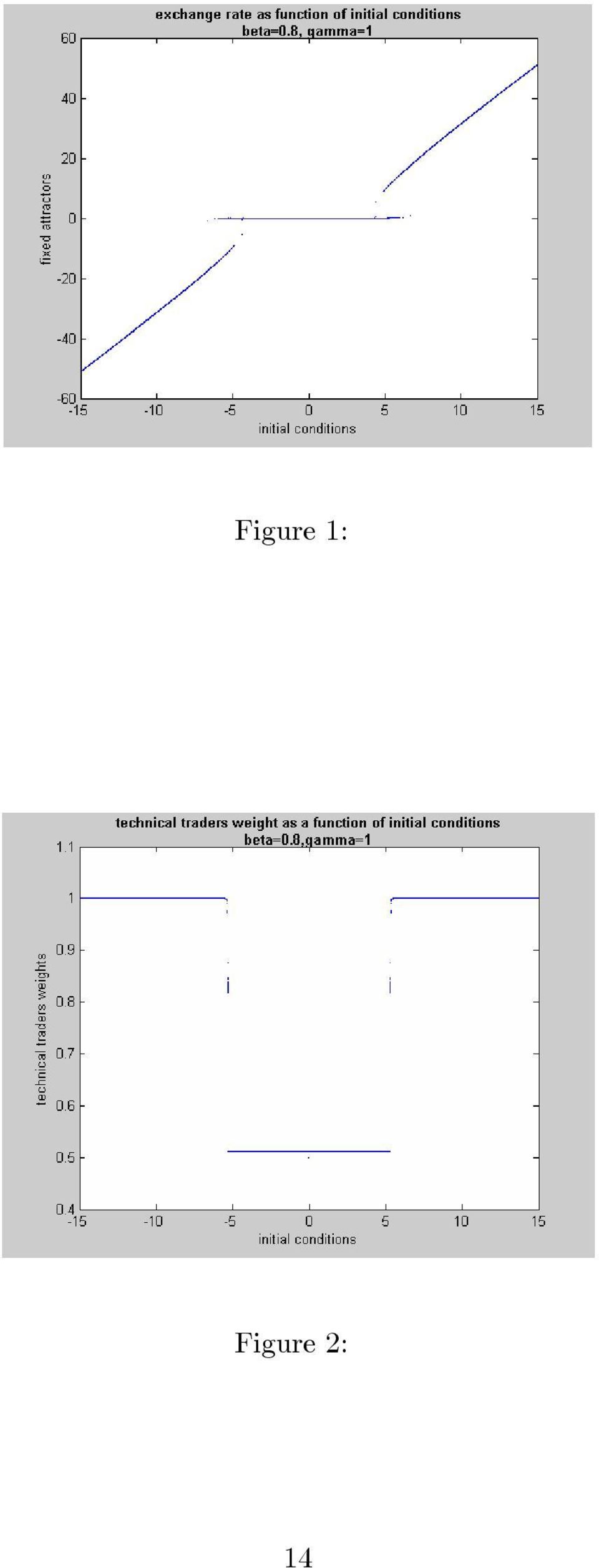
14 3.2 Numerical analysis The strong non-linearities make an analysis of the model s global stability impossible. Therefore, we use simulation techniques which we will present in this and the following sections. We select reasonable values of the parameters, i.e. those that come close to empirically observed values. In appendix we present a table with the numerical values of the parameters of the model and the lags involved. As we will show later, these are also parameter values for which the model replicates the observed statistical properties of exchange rate movements. We will also analyse how sensitive the solution is to different sets of parameter values. The dynamical model used in the numerical analysis is the same one as in the previous section except for the number of lags in the technical traders forecasting rule. We now return to the specification of the technical traders s rule as given by 8. As a result, (13) becomes s t = s t 1 Θ f,t ψs t 1 + Θ c,t β TX α i s t i where T = 5. Thus, the full model with all its lags is a 10-dimensional dynamic system. In figure 1 we show the solutions of the exchange rate for different initial conditions. On the horizontal axis we set out the different initial conditions. These are initial shocks to the exchange rate in the period before the simulation is started 11. The vertical axis shows the solutions corresponding to these different initial conditions. These were obtained from simulating the model over periods. We found that after such a long period the exchange rate had stabilized to a fixed point (a fixed attractor). The fundamental exchange rate was normalized to 0. Wefind the two types of fixed point solutions that we discussed in the previous section. First, for small disturbances in the initial conditions the fixed point solutions coincide with the fundamental exchange rate. We call these solutions the fundamental solutions. Second, for large disturbances in the initial conditions, the fixed point solutions diverge from the fundamental. We will call these attractors, bubble attractors 12. It will become clear why we label these attractors in this way. The larger is the initial shock (the noise) the farther the fixed points are removed from the fundamental exchange rate. The border between these two types of fixed points is characterised by discontinuities. This has the implication that in the neighbourhood of the border a small change in the initial condition (the noise) can have a large effect on the solution.we return to this issue. The different nature of these two types of fixed point attractors can also be seen from an analysis of the technical traders weights that correspond to these different fixed point attractors. We show these technical traders 11 There are longer lags in the model, i.e. five Thus we set the exchange rate with a lag of more than one period before the start equal to 0. This means that the initial conditions are one-period shocks in the exchange rate prior to the start of the simulation. All the other lagged dynamic variables are set equal to 0 when the simulation is started. 12 We use the word bubble in a different way than in the rational expectations literature. We discuss this in a later section. i=1 12

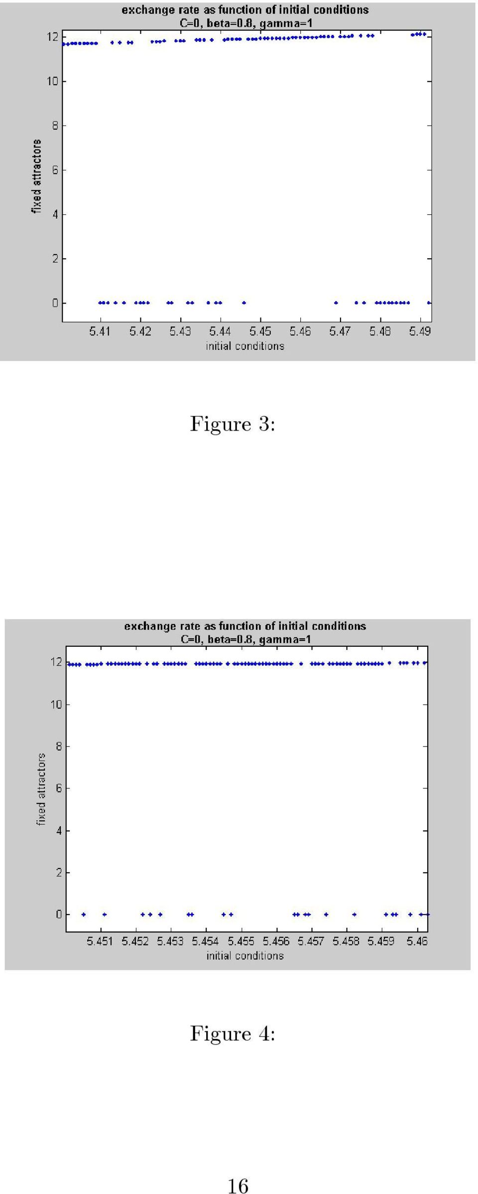
15 weights as a function of the initial conditions in figure 2. We find, first, that for small initial disturbances the technical traders weight converges to 50% of the market. Thus when the exchange rate converges to the fundamental rate, the weight of the technical traders and the fundamentalists are equal to 50%. For large initial disturbances, however, the technical traders weight converges to 1. Thus, when the technical traders take over the whole market, the exchange rate converges to a bubble attractor. The meaning of a bubble attractor can now be understood better. It is an exchange rate equilibrium that is reached when the number of fundamentalists has become sufficiently small (the number of chartists has become sufficiently large) so as to eliminate the effect of the mean reversion dynamics. It will be made clearer in the next section why fundamentalists drop out of the market. Here it suffices to understand that such equilibria exist. It is important to see that these bubble attractors are fixed point solutions. Once we reach them, the exchange rate is constant. The technical traders expectations are then model consistent, i.e. technical traders who extrapolate the past movements, forecast no change. At the same time, since the fundamentalists have left the market, there is no force acting to bring back the exchange rate to its fundamental value. Thus two types of equilibria exist: a fundamental equilibrium where technical traders and fundamentalists co-exist, and a bubble equilibrium where the technical traders have crowded out the fundamentalists 13. In both cases, the expectations of the agents in the model are consistent with the model s outcome. These two types of equilibria differ in another respect. The fundamental equilibrium can be reached from many different initial conditions. It is locally stable, i.e after small disturbances the system returns to the same (fundamental) attractor. In contrast there is one and only one initial condition that will lead to a particular bubble equilibrium. This implies that a small disturbance leads to a displacement of the bubble solution. Note also that the border between these two types of equilibria is characterized by discontinuities and complexity, i.e. small disturbances can lead to either a fundamental or a bubble equilibrium. We show the nature of this complexity in the figures 3 and 4. These present two successive enlargements of figure 1 around the initial condition, 5, where the fundamental and bubble equilibria appear to overlap. We observe that small changes in the initial conditions can switch the equilibrium point from a fundamental to a bubble equilibrium, and vice versa.the second enlargement shows the replicating nature of the enlargements. The holes in the line segment describing the fundamental equilibrium in the first enlargement are now filled up with fundamental equilibria that were not visible in the first enlargement. Thus, we find that in the border region between fundamental and bubble equilibria there is sensitivity to initial conditions, i.e. trivially small shocks can lead to switches in the nature of the equilibrium to which the exchange rate is attracted. This also suggests that these fixed point attractors are surrounded 13 Note that the intermediate points, i.e. when chartists weight is less than 1 the solution has not converged yet to fixed points. Fundamentalists hold a very small share in the market which exerts some mean reverting force. However their influence is offset by the chartists pressure. In figure 2 the simulation results are for T=

16 Figure 1: Figure 2: 14

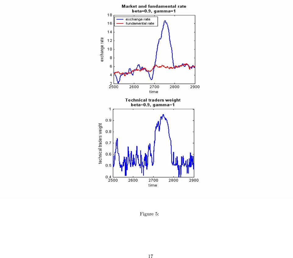
17 by basins of attraction that are separated by complex borders. We will return to informational issues produced by this result. 4 The anatomy of bubbles and crashes In the previous section we identified the existence of two different types of fixed point solutions, i.e. a fundamental solution characterised by the fact that the exchange rate converges to its fundamental value while technical traders and fundamentalists co-habitate, and a bubble solution in which the exchange rate deviates from its fundamental value and in which technical traders dominate the market. In this section we show that in combination with stochastic shocks in the fundamental exchange rate these features of the model lead to the emergence of bubbles and crashes. Again we selected a particular set of parameter values. In section 5 we present a sensitivity analysis. We start by presenting a case study of a typical bubble and crash scenario as produced by the stochastic version of the model. Figure 5 top panel shows the exchange rate and its fundamental value in the time domain; the bottom panel showstheweightofthechartistsinthesametimedomain.thesetwopictures allow us to analyse a number of common features of a typical endogenously generated bubble and crash in a stochastic environment. First, once a bubble emerges, it sets in motion bandwagon effects. As the exchange rate moves steadily in one direction, the use of extrapolative forecasting rules becomes more profitable, thereby attracting more technical traders in the market. This is clearly visible from a comparison of the bottom panel with the top panel of figure 5. We observe that the upward movement in the exchange rate coincides with an increase in the weight of technical traders in the market. We have checked this feature in many bubbles produced by the model. In appendix 1 we show another example of a bubble, and we present the results of a causality test ( correct it according to uppsala) which shows that the exchange rate leads the weight of technical traders during a bubble and the subsequent crash. Thus, typically a bubble starts after the exchange rate has moved in one direction, thereby attracting extrapolating technical traders which, in turn, reinforces the exchange rate movement. Second, a sustained upward (downward) movement of the exchange rate will not develop into a full scale bubble if at some point the market does not get sufficiently dominated by the technical traders. As can be seen figure 5 at the height of the bubble the technical traders have almost 100% of the market. Put differently, an essential characteristic of a bubble is that at some point most agents are not willing to take a contrarian fundamentalist view. The market is then dominated by agents who extrapolate the bubble into the future. This raises the question of why fundamentalists do not take an opposite position thereby preventing the bubble from developing. After all, the larger the deviation of the exchange rate from the fundamental the more the fundamentalists expect to make profit from selling the foreign currency. Yet they do not, and massively 15

18 Figure 3: Figure 4: 16

19 Figure 5: 17

20 leave the marketplace to the technical traders. The reason is twofold. First, during the bubble phase the profitability of technical trading increases dramatically precisely because so many technical traders enter the market thereby pushing the exchange rate up and making technical trading more profitable. Second, during the bubble phase fundamentalists make large forecasting errors, reducing their appetite for using fundamentalists forecasting rules. Put differently, during the bubble phase the riskiness of taking a fundamentalist position (as measured by forecast errors) increases dramatically relative to the riskiness of extrapolative forecasting. As a result, of these two effects fundamental investors who are continuously acting against the trend will tend to drop out. There is therefore a self-fulfiling dynamics in the profitability of technical trading and losses for the fundamentalists. The limit of this dynamics is reached when technical traders have crowded out the fundamentalists. We arrive at our next characteristics of the bubblecrash dynamics. When the technical traders share is close to 100% the selfreinforcing upward movement in the exchange rate and in profitability slows down, increasing the relative profitability of fundamentalists. An exogenous shock, e.g. a shock in the fundamental, can then trigger a fast decline in the share of technical trading, back to its normal level of a tranquil market. A crash is set in motion. We come back to issue of why a crash must necessarily occur in this model. The dynamics of bubbles and crashes we obtain in our simulated data is asymmetric, i.e. bubbles are relatively slow and crashes relatively rapid. An intuitive explanation of this result is that during a bubble technical traders and fundamentalists rules push the exchange rate in two different directions, i.e. the positive feedback from technical traders and the negative feedback from fundamentalists have the effect of slowing down the build-up of a bubble. In a crash the fundamentalists mean reverting force is reinforced by the technical traders behaviour. As a consequence, the speed of a crash is higher than the speed with which a bubble arises. This asymmetry between bubbles and crashes is a well-known empirical phenomenon in financial markets (see Sornette(2003)). In figure 6 we present the DEM-USD for the period , which is a remarkable example of a bubble in foreign exchange markets. As it can be seen from figure 6 the upward movement in the DEM-USD exchange rate is gradual and builds up momentum until a sudden and much faster crash occurs which brings the exchange rate back to its value of tranquil periods. Our model provides a simple explanation for this empirical phenomenon Note the contrast with rational expectations models of bubbles and crashes. These predict that bubbles and crashes are symmetric (Blanchard(1979) and Blanchard&Watson(1982)) Moreover,thesymmetryofbubblesandcrashesneglectsthetimescaledynamicsinwhicha long term change is an accumulation of short term changes. Thus, the symmetry property in foreign exchange markets is an approximation which holds only in the (very) short-run (see Johansen and Sornette (1999)). 18

21 DEM-USD Figure 6: 5 Sensitivity analysis: the deterministic model In this section we perform a sensitivity analysis of the deterministic model. This will allow us to describe how the space of fundamental and bubble equilibria is affected by different values of the parameters of the model. In this section we concentrate on two parameters, i.e. β (the extrapolation parameter of technical traders) and γ (the sensitivity of technical traders and fundamentalists to relative profitability). 5.1 Sensitivity with respect to β We show the result of a sensitivity analysis with respect to β in figure 7, which is a three-dimensional version of figure 1. The fixed attractors (i.e. the solutions of the exchange rate) are shown on the vertical axis. The initial conditions are shownonthex-axisandthedifferent values for β on the z-axis. Thus, the twodimensional figure 1 in section 3 is a slice of figure 7 obtained for one particular value of β (0.8 in figure 1). We observe that for sufficiently low values of β we obtain only fundamental equilibria whatever the initial conditions. As β increases the plane which represents the collection of the fundamental equilibria narrows. At the same time the space taken by the bubble equilibria increases, and these bubble equilibria tend to increasingly diverge from the fundamental equilibria. Thus as the extrapolation parameter increases, smaller and smaller shocks in the initial conditions will push the exchange rate into the space of bubble equilibria. Put differently, as β increases, the probability of obtaining a bubble equilibrium increases. 19

22 Note also that the boundary between the fundamental and the bubble equilibria is a complex one. The boundary has a fractal dimension. We return to this issue in section Sensitivity with respect to γ The parameter γ is equally important in determining whether fundamental or bubble equilibria will prevail. We show its importance in figure 8, which presents a similar three-dimensional figure relating the fixed attractors to both the initial conditions and the values of γ. We find that for γ =0or close to 0, all equilibria are fundamental ones. Thus, when agents are not sensitive to changing profitability of forecasting rules, the exchange rate will always converge to the fundamental equilibrium whatever the initial condition. As γ increases, the space of fundamental equilibria shrinks. With sufficiently high values of γ, small initial disturbances (noise) are sufficient to push the exchange rate into a bubble equilibrium. Put differently, as γ increases, the probability of obtaining a bubble equilibrium increases. Finally, as in the case of β, we also observe that the boundary between the bubble and fundamental equilibria is complex. 6 The frequency of bubbles In the previous section we described the zones of attraction around fundamental and bubble equilibria in a deterministic environment. In a stochastic environment the exchange rate will constantly be thrown around in these different zones of attraction. It is threfore useful to simulate the model in a stochastic environment to find out how frequently the exchange rate will be attracted by bubble equilibria. We analyse this issue by simulating the stochastic version of the model and by counting the number of periods the exchange rate is involved in a bubble. We define a bubble here to be a deviation of the exchange rate from its fundamental value by more than three times the standard deviation of the fundamental variable for a significant interval of time. We have set this interval equal to 20 periods. We show the result of such an exercise in figure 9 for different values of the chartists extrapolation parameter β and the rate of revision γ. It shows the percentage of time the exchange rate is involved in a bubble dynamics. We observe that when β and γ are small the frequency of the occurrence of bubbles is small. The frequency of bubbles increases exponentially with the size of the parameters β and γ. Thus, the extrapolation by chartists β and the rate of revision γ are important parameters affecting the frequency with which bubbles occur. The previous results allow us to shed some additional light on the nature of bubbles and crashes. As we have seen before, bubbles arise because agents are attracted by the risk-adjusted profitability of the extrapolating (technical traders) rule, and this attraction in turn makes this forecasting rule more profitable, leading to a self-fulfilling increase in risk-adjusted profitability. For this 20

23 Figure 7: Figure 8: 21

24 Figure 9: dynamics to work, agents decision to switch must be sufficiently sensitive to therelativerisk-adjustedprofitabilities of the rules. If it is not the case, no bubble equilibria can arise. The larger is γ themorelikelyitisthattheseselffulfilling bubble equilibria arise. The interesting aspect of this result is that in a world where agents are very sensitive to changing profit opportunities, bubbles become more likely than in a world where agents do not react quickly to these new profit opportunities Permanent shocks and bubbles In his classic book Manias, Panics, and Crashes. A History of Financial Crises Kindleberger identifies one source of the emergenence of bubbles in the stock markets to be a shock such as a technological innovation or an institutional change that affect the the long run profitability prospects of firms. We checked whether this historical analysis of the emergence of bubbles is mimicked in our model. The way we did this is to assume that a positive and permanent shock occursinthefundamentalvalueoftheassetprice(theexchangerate).weset this shock equal to +4. It occurs at the start of the simulation. We then analysed the solutions of the exchange rate for different initial shocks (noise) and for different values of β. The results are shown in figure 10. We have indicated the 15 The policy implication of this result is that by increasing the inertia in the system so that agents react less quickly to changes in relative profitabilities of forecasting rules, the authorities could reduce the probability of the occurrence of bubbles. How this can be done and whether some form of taxation of exchange transactions can do this, is a question we want to analyse in future research. 22

25 new and permanent value of the fundamental exchange rate by the vertical plane through +4. We observe an important asymmetry in the space of fundamental and bubble equilibria. Compared to the symmetric case of figure 7, the horizontal plane collecting the fundamental equilibrium has shifted to the left 16. This means that relatively small positive noise in the initial conditions leads to bubble equilibria for all values of β, while one needs large negative noise to obtain (negative) bubble equilibria. Thus the model predicts that when a positive shock occurs in the fundamental, the probability of obtaining a (positive) bubble equilibrium increases. Figure 10: This result may also explain why in stock markets positive bubbles appear to be more common than negative bubbles. In a growing economy, positive and permanent shocks in the fundamental occur more frequently than negative ones. Our model then predicts that in such an environment positive bubbles will arise more frequently than negative ones. Note that, in the foreign exchange market, a positive bias in the fundamental shocks is less likely to occur, because the fundamental exchange rate is the result of a differential between domestic and foreign variables. Thus, bubbles in the foreign exchange markets are more likely to be both negative and positive ones. 8 Why crashes occur The model makes clear why bubbles arise in a stochastic environment. It may not be clear yet why bubbles are always followed by crashes. Here again shocks 16 Note that the horizontal plane has also shifted upwards by +4, but this is not very visible. 23

26 in the fundamental are of great importance. In order to analyse this issue we performed the following experiment. We fixed the initial condition at some value (+5) that produces a bubble equilibrium (for a given parameter configuration). We then introduced permanent changes in the fundamental value (ranging from -10 to +10) and computed the attractors for different values of β. We show the resultsofthisexerciseinfigure 11. On the x-axis we show the different fundamental values of the exchange rate, while on the y-axis we have the different values of β. The vertical axis shows the attractors (exchange rate solutions). The upward sloping plane is the collection of fundamental equilibria. It is upward sloping (45%) because an increase in the fundamental rate by say 5 leads to an equilibrium exchange rate of 5. For low values of β we always have fundamental equilibria. This result matches the results of figure 7 where we found that for low β s all initial conditions lead to a fundamental equilibrium. The major finding of figure 11 is that when permanent shocks in the fundamental are small relative to the initial (temporary) shock, (+5) we obtain bubble equilibria. The corollary of this result is that when the fundamental shock is large enough relative to the noise, we obtain a fundamental equilibrium. Thus if an initial temporary shock has brought the exchange rate in a bubble equilibrium, a sufficiently large fundamental shock will lead to a crash. In a stochastic environment in which the fundamental rate is driven by a random walk (permanent shocks), any bubble must at some point crash because the attactive forces of the fundamental accumulate over time and overcome the temporary dynamics of the bubble. The interesting aspect of this result is that the crash occurs irrespective of whether the fundamental shock is positive or negative. Since we have a positive bubble, it is easy to understand that a negative shock in the fundamental can trigger a crash. A positive shock has the same effect though. The reason is that a sufficiently large positive shock in the fundamental makes fundamentalist forecasting more profitable, thereby increasing the number of fundamentlists in the market and leading to a crash (to the new and higher fundamental rate). Put differently, while in the short run, chartists exploit the noise to start a bubble, in the long run when the fundamental rate inexorably moves in one or the other direction, fundamentalists forecasting becomes attractive. It is also interesting to note that as β increases, the size of the shocks in the fundamental necessary to bring the exchange rate back to its fundamental rate increases. In a stochastic environment this means that bubbles will be stronger and longer-lasting when β increases. In conclusion, it is worth noting that shocks in fundamentals both act as triggers for the emergence of a bubble (see previous section) and as triggers for its subsequent crash. The intuition can be explained as follows. When the exchange rate is in a fundamental equilibrium, an unexpected and permanent increase in the fundamental, sets in motion an upward movement of the exchange rate towards the new fundamental. This is the result of the action by fundamentalists. This upward movement, however, also makes extrapolative forecasting (technical trading) increasingly profitable and can lead to a bubble. When the exchange rate is in a bubble equilibrium, a large enough (positive 24