The Decennial Pattern, the Presidential Cycle, Four- year Lows, and How They Affect the Stock Market Outlook for 2010

Transcription

1 The Decennial Pattern, the Presidential Cycle, Four- year Lows, and How They Affect the Stock Market Outlook for 2010 Since this is the start of the first year of a new decade it seemed like a good idea to examine a largely forgotten but useful concept known as the Decennial Cycle. As we delved deeper into this task and took into consideration the fact that 2010 is a 4-year cycle low and the second (most bearish) year of the Presidential Cycle, it became apparent that this year could be quite a challenging one for the equity market. Bearing in mind there is usually a happy ending to all this, let s consider each of these concepts in turn. The Decennial Cycle The Decennial pattern was first noted by Edgar Lawrence Smith, who in 1939 published a book called Tides and the Affairs of Men. 3 His previous work, Common Stocks as a Long Term Investment, had been a best-seller in the late 1920s. 4 Smith researched equity prices back to 1880 and came to the conclusion that a 10-year pattern, or cycle, of stock price movements had more or less reproduced itself over that 58-year period. He professed no knowledge as to why the 10-year pattern seemed to recur, although he was later able to correlate the decennial stock patterns with rainfall and temperature differentials in Common Stocks and Business Cycles. Even though the cycle has been relatively reliable there has been to date no rational explanation as to why it works. Smith used the final digit of each year's date to identify the year in his calculations. He termed the years 1881, 1891, 1901, etc., as the first years; 1882, 1892, etc. are the second; and so forth. Inspired by the research of Dr. Elsworth Huntington and Stanley Jevons, who both emphasized the 9- to 10-year periods of recurrence in natural phenomena, Smith experimented by cutting a stock market chart into 10-year segments and placing them above each other for comparison. These various decades are displayed individually in Appendix A. A secular bull trend is one in which stock prices experience a persistent up trend over the course of several 1

2 business cycles. A secular bear is the opposite, although some become trading ranges as opposed to an actual bear market. Chart 1shows three series, those averaged for decades in which there was a secular bull market (e.g.1990 s), those that developed under the cloud of a secular bear (e.g.1930 s), and an average of all decades since Chart 1 The green (secular bull) and the red (secular bear) contain different decades yet their trajectories are not that dissimilar. The pattern observed by Smith early in the twentieth century has not changed much since then. It still appears that a typical decade consists of three cycles, each lasting approximately 40 months. The 52-week ROC of the average decennial pattern (Chart 2) brings this cyclic rhythm out well, with lows generally appearing in years two, four and seven/early eight and highs in three, six and nine. In this exercise the year ending in zero is regarded as the tenth year. 2

3 The 2000 s vs. the Average Decennial Cycle Charts 2 and 3 compare the latest decade with the average. In Chart 2 this is the average of all decades, while Chart 3 represents the average of all decades that developed in a secular bear market environment. You can also see that this is not a perfect science because the ROC for the 2000/09 decade in Chart 2 fails abysmally to follow the idealized average pattern except for early decade weakness and the mid 2007 peak. Going into 2010 however, the ROC is consistent with an overbought condition at a reading of +25%. That does not forecast a decline into 2010 but definitely places the market in a more vulnerable situation than if the reading was below zero. Chart 2 3

4 Chart 3 For example in 1949, the ROC was very oversold and was inconsistent with its normal position in the decennial pattern. Instead of declining into 1950, the market actually rose. This experience is a good example of why the decennial approach should be used with other technical indicators and not in isolation. Perhaps of greater importance is the fact that the market at the close of 1949 represented excellent value in terms of dividend yield and P/E ratio and had just emerged from a recession. There really was only one way it could go! Chart 3 highlights those turning points where the 2000/09 decade developed in sympathy with the average. This series certainly cannot be used as a precise timing device because it indicated strength between mid 2008 into early 2009, whereas the actual experience was extreme weakness. That s why any study such this cannot be carelessly extrapolated but must be used in conjunction with many other indicators. 4

5 Years Ending in Zero According to Smith s analysis years ending in a seven were the worst with the fifth being the best performer. However, it could be argued, based on the consistency of losses, that years ending in zero are even more challenging. Appendix B shows the weekly path of the Dow for all zero years since, where we see four up and seven down. Chart 4 The character of the year depends a lot on whether it takes place during a secular bull or bear market. Up until late August there is not much difference in terms of the wave patterns. 5

6 After that a late year-end rally lifts the secular bull average to a positive return, but pushes the average secular bear to an even worse performance. One consistent characteristic is that after a weakfish opening and subsequent rally the late March/April period ushers in a universally negative environment. Table 1 sets this out quite clearly because every year experiences a midsummer low below that of the January opening price. The average decline was a stunning 14%. The average loss at the mid-year lows was actually greater than that at year-end because of the strong the upward bias from September onwards in secular bullish years as well as strong year end rallies in 1970 and Year Open Close Mid yr Low Date Year Loss Mid Year Loss Jun Jul May Jun Jun Jul Apr May Apr Apr Mar Average Table 1 Smith never offered a rationale as to why years ending in a zero were so weak. However, with the benefit of hindsight it is apparent that most of these instances have been associated with recessions. Specifically these were 1900, 1910, 1920, 1930, 1960, 1970, 1980 and 1990.The year 2000 was not a recession one but led the 2001 downturn. Similarly, the bear year of 1940 was associated with WWII. The 1950 experience was preceded by a recession in 1949, so the market had every reason to go up, which it did. As a result zero year weakness can be pretty well explained by negative economic conditions. 6

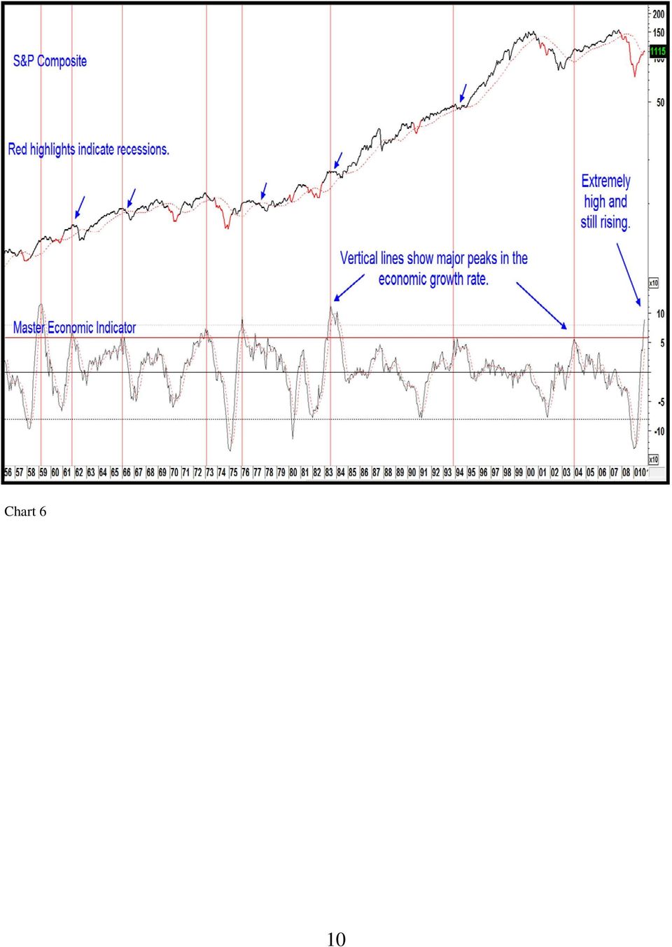
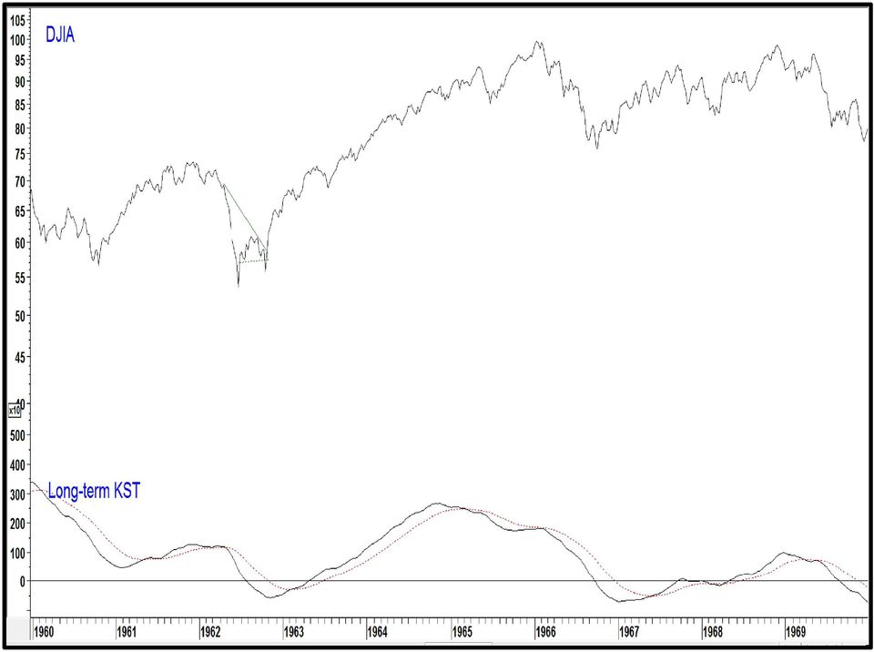
7 The Presidential Cycle The rationale for this concept is that the election year experiences economic stimulus as the party in power seeks to keep voters in good spirits. The first year of the cycle, the inauguration year, benefits from this and is therefore positive for equities. However, the second year sees a tightening in policy as the authorities seek to reign in the inflationary pressures now beginning to build. An alternative scenario holds that the stock market is sensitive to the growth path of the economy. Consequently, as the election year stimulus effect wears off, the economic growth path starts to decline and stocks suffer. Such was the case in 1962 and The facts support the theory, because year two of the cycle has been statistically the worst performer. This year just happens to be another second year in the Presidential cycle. Four Year Cycle Low The good news is that the second year of the Presidential Cycle also corresponds with the so called four year cycle low. Chart 5 flags these points with the arrows. And you can see that they generally offer good buying opportunities. In 1925, 1934, 1986 and 2006 these excellent acquisition points developed within a strong uptrend. It is interesting to note that each of these years was associated with a slow-down in the economic growth rate, but not an actual recession. Normally, there is a greater chance that these buying opportunities will be earned, since they are typically preceded by a nasty decline. You may have wondered why the arrows are not equidistant from each other since this is, after all, a four year cycle. The reason is that the buying points do not develop at the same time each year. Indeed during the 1922, 1918, 1950, 1954 and 1958 cycles the actual low formed late in year prior to that in which the four year low was due to appear, probably because these lows were associated with the end of a recession, in effect, clearing the way for stock prices in the year of the idealized cycle low to advance. Only in 1918 does the recession argument not hold. The line of reasoning in this case would be that the 1917 low came early because the market was in a hurry to discount the end of World War I. At William Hester notes that since 1933 the average January/September period for the second year of the cycle has basically been flat, as up years have roughly equaled down years but some of the down years have been quite strong. He 7

8 cites 1962, 1974 and more recently 2002 as examples. However, the good news is that the second presidential year average fourth quarter gain has been 8.7%. It gets better, as he goes on to point out that the fourth quarter of the second year is actually where many third-year (Presidential cycle) rallies are born. His research shows that the 12-months that include the fourth quarter of year two and the first three quarters of year three have enjoyed average total returns of more than 28 percent. Since 1933 not a single such 12-month period has registered a loss, the worst return being a gain of 6.6%. Chart 5 8

9 The Year Ahead There is obviously no known method of forecasting what precisely lies ahead, but based on the history of the interaction of the Decennial, Presidential Cycles, four-year cycle lows and the assumption that we are still in a secular bear market, it s possible to come up with three generalizations. First, based on our knowledge of the opening year of the decade, it is likely that a peak of some kind is likely to develop in the 6-weeks following the middle of March as a very strong negative seasonal tendency gets underway. History shows that equity price trends leading into the spring have been varied with a downward bias. All we can say for sure is that the intermediate KST for the S&P has recently triggered a sell signal from an overbought position. That reduces, but certainly does not eliminate, the odds of an extension of the recent rally into the spring. The second point is that most of these cycle lows were either associated with declines in the economic growth rate or actual contractions. In situations where growth slowed but did not contract, equity price weakness was much less pronounced. Since the economy has just emerged from a deep recession and monetary policy is still accommodative, there seems little reason, barring an unexpected shock to the system, for expecting another recession in the immediate future. However, our Master Economic Indicator (MEI), which correlates well with stock prices, is currently at an extremely high reading (see Chart 6). It s still rising of course, but its upward trajectory is clearly unsustainable. One third of its components are based on a 9-month rate-ofchange, and since many of them bottomed last March and April only a sharp acceleration in the months ahead will avoid a peaking in the MEI itself. Chart 6 also shows that the corrections that took place in 1962, 1966, 1978, 1984, and 1994 were all associated with a peaking in the MEI but there was no recession. These periods have been flagged by the small blue arrows. The confluence of cyclic forces discussed above and their close correlation with economic activity suggests that this year will experience a moderate 10-20% to correction unless the economy falls back into recession, a development on which we place relatively low odds. Although the correction could begin at anytime, the most vulnerable period will begin from late March on. The final observation is that the fourth quarter of the second Presidential Year is typically strong and represents an ideal time for a four-year cycle buying opportunity. While the low could well be set earlier than that, the most ideal time would be the October/November period. Since the 12-months following the end of the third quarter of the second year are historically and consistently buoyant, the year 2011 is setting up to look better than

10 Chart 6 10

11 Appendix A Decennial Patterns Since 1900

12

13

14

15

16

17

18

19

20

21

22

23 Appendix B Opening Years of the Decade

24

25

26

27

28

29