Video codecs in multimedia communication

Transcription

1 Video codecs in multimedia communication University of Plymouth Department of Communication and Electronic Engineering Short Course in Multimedia Communications over IP Networks T J Dennis Department of Electronic Systems Engineering, University of Essex tim@essex.ac.uk Fundamentals of Digital Pictures The idea of 'Bandwidth' Resolution Human factors Compression for still images: JPEG/GIF Compression for Motion: Fundamentals of Interframe Coding Videoconferencing: H.261/H.263 Low-end video applications: MPEG-1 High quality (broadcasting): MPEG-2 Introduction to 'Multimedia objects': MPEG-4 Principal reference: Video coding, an introduction to standard codecs, M Ghanbari, IEE 1999.

2 Human Factors 'Bandwidth' in Electronic Communication Bandwidth is the range of frequencies needed to transmit to get a 'satisfactory' reproduction of a signal, which will usually be analogue at both ends. In digital systems it relates to the number of bits per second that have to be sent. Exactly how this is done is the concern of the lowest physical and transport layers of the standard model. In the case of binary signalling, the 'analogue' bandwidth of the digital signal may be many times that of the analogue source itself - for example, telephone speech as two-level PCM needs 32 khz for a 3.4 khz signal! However, a combination of sophisticated signalling methods, e.g. COFDM in the case of terrestrial digital TV, and compression algorithms like MPEG mean that one 8 MHz analogue UHF TV channel can now carry 32 or 64 Mbit/sec, and 6 or more TV programs. General Examples System Raw Analogue Transmitted Digital Bitrate Bandwidth Analogue (Pulse Code Bandwidth Modulation) Telephone 3 Hz khz (same) 64 kbit/s AM Radio 5 Hz - 4 khz 8 khz N/A FM Radio 5 Hz - 13 khz 2 khz N/A TV sound NICAM 5 Hz - 15 khz N/A 728 kb/s Digital Stereo TV sound Digital Pictures Source Picture size Compression Compressed size/ (8-bit samples) Method data rate Single e.g = JPEG 15-3 kbytes image 37 kbytes (typ. 5-2% of raw) Motion Broadcast: MJPEG 1 mbyte = video "Motion 8 Mb/s 25 pix/sec = JPEG" 1 Mbytes/s do. do. MPEG Mb/s Compact Disk 5 Hz - 2 khz N/A 1.4 Mb/s (stereo) PAL Colour TV Hz MHz 8 MHz (AM) 2 Mb/s 27 MHz (FM) 2

3 Picture Resolution 1. Simulation of 3 lines, 1:2 aspect ratio, vertical scanning. This is the kind of image obtained by Baird in the earliest broadcast trials of the 193s. It used a picture rate of 12 1 / 2 per second (he did manage to reproduce colour experimentally!). 2. An actual 3 line image decoded by Don McLean from an audio disk recording made between 1932 and 1935 from a BBC broadcast (see for further examples). 2 (This image is copyright D.F. McLean 1998) 1 3

4 Picture Resolution lines, 4:3 aspect ratio, horizontal scanning. About the best quality achievable by real-time mechanical scanning. 3 4

5 Picture Resolution lines, 4:3 aspect ratio. Equivalent to the current 625 line analogue standard 4 5

6 Human Factors Brightness Perception: which of the small squares is lightest? The true situation is revealed by bringing the small squares close together: 6

7 'Spatial Frequency' Patterns periodic in space 1 Contrast Sensitivity 1 1 From Transmissio and Display of Pictorial Information, Pearson 1975 Visual spatial frequency response Low luminance High luminance Spatial Frequency (cycles/degree) 7

8 Two-Dimensional Fourier Spectra (log amplitude is shown) The centre of each spectrum corresponds to spatial frequency (,), or the mean DC level 8

9 Visual frequency response test pattern Spatial frequency increases logarithmically from left to right, while the contrast increases from bottom to top. Draw an imaginary line where the sinusoid just becomes detectable. Depending on viewing distance, there should be a definite peak somewhere near the centre. 9

10 Sensitivity to temporal variation 5 High light levels From Transmission and Display of Pictirial Information, Pearson Contrast sensitivity 1 Low light levels Frequency (Hz) Visual flicker sensitivity 1

11 Interactions: masking (The real world is a lot more complicated...) 11

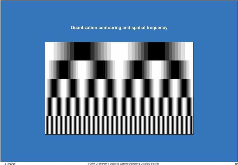
12 Quantization contouring and spatial frequency 12

13 Dealing with Colour A very important aspect of human colour vision strongly affects the amount of compression that can be applied to colour images. It has been exploited, probably unwittingly, by artists and relates to an inability to perceive fine detail in the colour content of a scene. The eye is sensitive to high-spatial frequency luminance, but not to a similar pattern where two colours of the same luminance are closely interleaved. To make use of this phenomenon, colour pictures for transmission or compression are converted from red, green and blue (RGB) to a different set of coordinates: luminance (what a black-and-white camera would see) and colour difference or chrominance signals. For example, in broadcast TV the signals actually transmitted are: Luminance, Y =.3R +.59G +.11B Red colour difference, C1 = V = R - Y Blue colour difference, C2 = U = B - Y (At the receiver, the missing G - Y signal can be derived from U and V, and hence R, G and B recovered for the display). The bandwidth (bitrate) allocated to the Y signal is the maximum the channel can accommodate, but the bandwidths of U and V can be greatly reduced without seriously affecting the perceived quality of the recovered image at the display. Hence instead of needing three times the bandwidth (compared with monochrome) for a colour picture, the system can get away with between 1 and 2 times the bandwidth. Original colour picture (see next pages for details) 13

14 Colour picture in Lab component form. ('Lab' is another colour coordinate system. Same principle as YUV) These illustrate another useful feature of chrominance representation, which is that for typical 'natural' scenes containing few areas of saturated colour, the colouring signals are of low amplitude Luminance, 'L' component 'a' colour component; handles colours on a red-cyan axis 'b' colour component; handles colours on a blue-yellow axis 14

15 Effects of differential bandwidth reduction Left: luminance only Below: chrominance only (for information, the lowpass filter is Gaussian, radius 2 pixels) 15

16 Digital Pictures Conversion to digital form involves two processes: Amplitude Quantization: The signal is represented as a series of discrete levels rather than a continuously varying voltage. Typically 256 are sufficient, leading to 8 bits per signal sample. (Compare this with high quality audio signals which need 16 or more bits per sample). Sampling: A real-time video signal is sampled in time at a rate at least 2 its analogue bandwidth. In practice, rates up to 15 MHz are used. Also, the sampling rate should be an integer multiple of the line scan frequency, khz (why?). For static images on a mechanical scanner a scanning density ('dots per inch') appropriate to the image resolution should be used. (Sampling and quantization are done simultaneously in the analogue to digital converter) Once in digital form, processes that are impossible or very difficult to do to the analogue version of the signal become feasible, and can be implemented in real-time by fast computer software or special digital hardware. For example: Standards conversion between 6 Hz and 5 Hz field rate systems (525 and 625 lines) Noise reduction A huge range of special effects, e.g. colour distortion, rotation, warping... Compression There are two main compression standards in use today for 'natural' images: JPEG for single frames and MPEG for moving images like broadcast TV. JPEG works by removing spatial redundancy in the image, which it does by transforming small blocks into a relative of the Fourier transform, the Discrete Cosine Transform (DCT). This is followed by a complex quantization process, which also involves statistical compression. JPEG can compress an image to around 1% of its raw size, with barely visible distortion. It is used very commonly for pictures on the Internet. MPEG removes some spatial, but mainly temporal redundancy: because not all of the picture changes from frame to frame, only the parts that do change need to be transmitted. MPEG uses motion compensation to track moving objects, and the DCT again to help with quantization. It can compress a moving TV image to about 1 megabit / second with some quality degradation, and to 4 Mb/s with almost no visible distortion. 16

17 Increasing Spatial Resolution Increasing Amplitude Resolution Spatial vs. Amplitude resolution In this picture, the amplitude and spatial resolutions increase as shown. The number of samples (left to right) is: 25 25, 5 5, 1 1 and 2 2. The number of quantizer levels (top to bottom) is 2 (1 bit per sample), 4 (2 bits), 16 (4 bits) and 256 (8 bits). The original is in colour, with red, green and blue quantized separately. 17

18 Data Compression The huge amounts of digital data needed to represent high-quality audio, video or single images make the use of raw PCM as the network transmission method impractical in many situations. For audio the problem is less severe, hence the success of CDs and NICAM digital TV sound. With pictures the raw data amounts (for still pictures) and rates (for motion video) are so great that compression of some kind is essential. The methods currently in use are the results of work over the past 3 years or so. Their practical implementation for real-time applications depends on the availability of very high-speed digital signal processing hardware; for example, the processing power needed to handle broadcast digital TV is comparable to that of a high-end PC, but the cost is of the order of 4. Compression factors are often expressed as the ratio of the input to output data; hence JPEG for single images gives about 1:1, while MPEG for video delivers 3-4:1. These methods are very effective, especially for video, and can deliver greatly improved quality (compared with analogue PAL) over a reduced channel bandwidth. Compression Fundamentals There are two basic methods: Lossless and Lossy. In practice they are used together to achieve compressions greater than can be obtained with either working alone. As the name implies, lossless methods introduce no distortion to the signal, meaning that the data sequence inserted at the input can be recovered exactly at the output. Lossy methods in contrast do introduce distortion, sometimes a considerable amount if measured in absolute 'mean squared error' terms. However, the distortion is carefully tailored to match the characteristics of the intended recipient receptor, eye or ear. The most important phenomenon that enables this to happen is masking as mentioned previously. Lossless Compression These methods all exploit statistical characteristics of the signal. A measure of how successful it is possible to be with a given source is given by its statistical entropy: 1 H = p i log 2 p i = p i log 2 all i all i p i where {p} are the probabilities of the i discrete 'symbols' emitted by the source. The entropy, H, gives the lower bound on the lossless compression possible on the source. 18

19 From the earliest days of 'digital' signalling, it was recognised that the way to achieve efficiency of transmission was to allocate short codewords to the most commonly occurring symbols. Hence the Morse code which allocates the shortest symbol (dot) to the letter 'E', which is the commonest, in English at least. In the case of binary signalling, we allocate variable numbers of bits to the various symbols to be transmitted in such a way that the bits per coded symbol depends inversely on the probability of the source symbols. Example This considers three possible codes for a set of 5 messages, together with some statistics of symbol usage: Message Number Possible variable length codes (VLCs) of occurrences X Y Z A=Hello 5 1 B=How are you? C=I'm fine D=I'm p***** off E=Please send file Total sample: 118 We can calculate the average number of bits per coded message, assuming the sample of 118 messages is representative, for each code. (Note that X is a fixed length code). Code X: Code Y: 3 bits/message ( )/118 = 25/118 = 2.17 bits/message Code Z: ( )/118 = 244/118 = 2.7 bits/message. Note that this is 69% of the bits needed by code X, a saving of 31% in transmission time per message on average. Decoding Bit stream: (1) Code X: E C C Code Y: D C B Code Z: B A A B A B Exercises 1. Calculate the entropy of the source. 2. How are codes Y and Z decoded? 3. What is the effect of a transmission error so that (say) the third bit is a 1 instead of zero? 19

20 Huffman Coding (lossless) Huffman's procedure to design a variable-length codebook generates one which is optimum in that it makes the average bitrate for the coded source as close as possible to the minimum, which is its statistical entropy. The procedure is conceptually very simple, and has three main steps. 1. Construct a 'probability flow' graph (right). In stage 1 the 'blocks' of probability, taken from the actual measurements, are ordered in descending size. The two smallest blocks are added together and the list of blocks, now one less is again rank ordered and passed to stage 2. This continues until stage 5 when we get a single number equal to the total number of measurements. 2. Arbitrarily label the branches where probabilities are combined with 1 or. In this example, there are 2 4 = 16 possible labellings. Message A B C D E Stage 1 (frequency) Stage Stage Stage Stage Read-off the codewords in reverse order, tracing the path of each block of probability from stage 1 to stage 5 and noting the label (1 or ) each time a branch occurs. This gives: A = B = 1 C = 11 D = 1111 E = 111 Hence the codewords as transmitted and interpreted by the decoder (assuming left-to-right order) for each symbol will be this set reversed: A = B = 1 C = 11 D = 1111 E = 111 2

21 It is easy to see intuitively why the code generates variable-length words in the way required: the smaller blocks of probability are going to be combined frequently, whereas the larger ones, like that for symbol A, remain intact for a greater number of stages. Receiving a Huffman code is very straightforward, and requires a simple treestructured sequence-detecting Finite State Machine (right), matched to the particular code of course: For each state of the machine, variable V indicates if there is a valid output Z, i.e. we are at a terminal state. Decoding of the next symbol from START then begins on receipt of the next incoming bit. Lossless compression for images START 1 V= V=1 Z=A 1 V= V=1 Z=B START 1 V= V=1 Z=C START 1 V=1 Z=D V=1 Z=E START START START The Huffman code can only provide some benefit (compression) if the input symbol set has an entropy significantly less than log 2 (number of symbols). What this means in practice is that its probability density function should be highly non-uniform or skewed. If we look at the pdf for the raw data from some typical images, it turns out that they generally do not have this property. One solution is to process the signal in a reversible way that results in a pdf of the desirable kind. This is one possibility that can exploit local (spatial or temporal) correlation within the picture. We generate a prediction of what the next incoming sample of the picture will be, then transmit a coded version of the error instead of the signal itself. At the receiver, for each sample the same prediction is made, but based on previously decoded samples, and the decoded error added to it: 8 bit video input + Σ Huffman coder Huffman decoder + Σ 8 bit video output Predictor + Transmission path Predictor 21

22 This shows a potential spatial predictor set for use with the system on the previous page. It calculates its 'guess' for element X by a weighted sum of elements A to C above and to its left. Scan directions Previous line B C D A X Current line Previous sample prediction. Above left: original image. Right: 'error' image obtained by subtracting the value of element A from the actual value of element X (A dc offset is added, so zero reproduces as mid grey). Below: pdfs corresponding to the images above. The entropy of the raw picture is 7.27 bits/ sample, while that of the prediction error is 5.28 bits. 22

23 Other predictors Which prediction is best to use depends on the picture content. It could, for example, change within the picture itself. Right is the error image for element C; the entropy is 5.38 bits/sample. Exercises 1. What must be done to the decoder, which the encoder must assume, before it starts to recover decoded signal values? 2. What is it about an image, or some area of it, that would suggest the use of a particular predictor? 3. Discuss the possible advantages and/or disadvantages of an adaptive prediction system for lossless image coding, and how it could be implemented. How would the choice of prediction be made? 4. The Huffman code can achieve compression that approaches the entropy asymptotically. The approximation is poor for small symbol sets (like the previous example) but improves for large ones. Why is this? It is fairly clear for these examples that the reduction in average bitrate to be obtained by lossless coding is not very great: about 2 bits per sample for this picture, or 25%. For pictures containing more detail the gain would be even less. Another approach is to take account of the characteristics of human vision, in particular the 'masking' phenomenon previously discussed and allow the compression process to introduce some distortion in such a way that it is visually insignificant. 23

24 Lossy image compression All high-compression coding methods introduce some distortion. One of the simplest methods of all is differential PCM, DPCM, which is again based on prediction, but using feedback rather than feed-forward as in the lossless case (Encoder above right; decoder below). DPCM works by generating a prediction as before, which can vary in complexity as required, then the error is quantized very coarsely. Whereas the error signal can, in theory, occupy the range ±255, and need 9 bits to represent it, the quantizer will reduce this (typically) to between 8 and 32 levels, needing 3 to 5 bits per sample for transmission (note that only an index of the quantized level is sent, not its actual value). At the receiver, the indexes are converted back to numerical values and added to the ideally identical prediction the receiver has made for that sample. Exercise Why is the feedback arrangement necessary for this system to work? 8 bit PCM input + Σ Prediction generator Prediction From channel decoder Prediction error Q Q 1 Local output Q 1 + Reverse quantizer + Σ Σ + To channel coder Quantized prediction error + Output The quantizer will usually have nonlinear step sizes, with most of the values concentrated near to zero. It is usually the case that an odd number of levels is desirable, which means that there can be a zero representative level as well. Picture quality is only weakly dependent on the exact design of the quantizer. Prediction generator The negative feedback structure of the encoder means that the prediction will always attempt to track the input whatever the source of perturbations, from the input signal or because of the quantizer. The diagram (right) shows an example of the behaviour of the local output for an input transition from zero to 63 with a 4-level quantizer having representative levels at ±3 and ±19. It is assumed that the initial prediction is also zero. Decoded output value Target level, etc DPCM step response Time 24

25 DPCM Performance The major artifacts of differentially coded images are slope overload, 'edge busyness' and granular noise. The first is exactly analogous to the slope-overload effect that occurs on operational amplifiers. It is caused by a too-small outer quantizer level, and affects sharp transitions that 'surprise' the predictor in use (as in the example on the previous page). Edge busyness in only visible on real-time coded images, and is a pattern of noise that again, affects sharp contrast changes as noise causes varying paths to be taken through the available quantizer steps. Granular noise appears in flat (low contrast) areas, and is caused by a too-large minimum quantizer level. It is more or less eliminated by having a zero level. Some of these effects are shown below. Original source image, uncompressed. Size is 256 by 256. The synthesised flat and ramp strips at the top indicate behaviour under low-contrast conditions. The white line tests impulse performance DPCM using 7 quantum levels,, ±5, ±1, ±15. Slope overload is the principal defect. Because the predictor is element A (previous element on the same line), vertical image features are most severely affected. 3. Associated error image, obtained by subtracting coded from original, and adding a 128 level dc offset. The peak signal to RMS 25

26 4. Same quantizer as picture (2), but using diagonal prediction, i.e. (A+C)/2. Now the distortion affects both horizontal and vertical features but is less severe in absolute amplitude. The SNR is only slightly improved at 22.6 db, but the subjective quality improvement is greater, confirming the unreliability of the SNR measurement. 7. Error image. 5. Error image 6. As (2) but using a quantizer with more widely spaced levels,, ±5, ±15, ±45. This greatly reduces slope overload, and improves the SNR to 28 db. Still poor, however. 8. Same quantizer as (6), but with (A+C)/2 predictor and simulated channel errors 26

27 Hybrid DPCM The compression performance of DPCM by itself is quite limited, with 16 or even 32 level quantizers being needed for fixed rate 4 or 5 bits/ sample coding. However, inspection of the typical usage of the quantizer levels shows that it is still highly nonuniform, indicating that a further saving might be possible by using a variable length code (VLC) on the quantizer index values. This is a typical result, after some experimentation with quantizer levels. The basic DPCM encoder uses a 17 level quantizer, which would require 4.9 bits/sample at fixed bitrate. Measuring the probability of occurrence gives these data for the same test image: Level Probability Note that the zero quantum level is used about 44% of the time. The entropy of this data set is bits/sample, which a Huffman VLC designed as previously should be able to approach quite closely. Above right is the output picture. It uses (A+C)/2 prediction and its SNR is 4.2 db, which is now good. Subjectively, the picture is even better, because the error affects detailed areas where masking plays a significant role. The close-ups are part of the original (left) and processed images. The error is most visible as noise in the shadow-road transition at the front of the car. The results with the simple experiment of combining the two techniques - DPCM and VLC - suggest that hybridisation has promise. Prediction with VLC, and DPCM alone give only moderate compressions, but combined they give a result that is better than both. This has proved to be a general principle in image coding, and probably applies elsewhere: it is best not to aim for huge compressions in a single stage, which frequently results in great complexity and difficulty of implementation. Use of two or more relatively simple methods is often the more effective approach. 27

28 Discrete Cosine Transform (DCT) The use of transforms in compression is an entirely different process from DPCM or the predictive statistical methods. Its aim is the same, however: to exploit local spatial correlations within the picture, and to exploit masking to conceal compression artifacts where they do occur. While it is in theory possible to deal with an image in its entirety, it is more usual, and practical, to work in small blocks. 8 by 8 is the most commonly used. Exercise Even if full-image transformation were practical, its performance is unlikely to be any better than the small-block implementation. Why is this? Mathematically, the assumption is that the image consists of rectangular (but usually square) blocks (matrices) X of correlated sample values. The idea is to transform X into another matrix Y, the same size, but where the elements are uncorrelated or have greatly reduced correlation. It then becomes possible to quantize each element individually. It can be shown theoretically that the transform which is maximally efficient at this process is the Karhunen-Loève Transform (KLT). This cannot be used in practice, because the transformation itself has to be recalculated for each incoming block. Instead, experiment has shown that the Discrete Cosine Transform is only marginally less efficient than the KLT, and very straightforward to compute. The DCT is used in both the JPEG and MPEG image compression algorithms. The DCT is closely related to the Discrete Fourier Transform, but requires only one set of orthogonal basis functions for each 'frequency'. For the one-dimensional case, i.e. a block of N 1 picture elements, the forward DCT is defined as: N 1 y [ ]= 2 N. x[ n] ; yk [ ]= 2 N and reverse: n= N 1 n= ( ) kπ 2n + 1 xn [ ].cos, k = 1 to N -1 2N N 1 xn [ ]= 1 2 y kπ 2n + 1 [ ]+ yk [ ].cos, n = to N -1 2N k =1 ( ) Just as for the DFT, 'fast' versions of this can be devised for block lengths that are powers of 2. 28

29 The DCT in Two Dimensions The DCT concept can easily be extended to two (or more) dimensions, in which case it is evaluated in exactly the same way as the DFT: as a series of 1-D transformations, say along the rows of an image block. The sets of transformed coefficients are then processed vertically in the same way, leading to a set of N 2 coefficients for a block of size N by N. What do the coefficients actually represent? This can be worked out by feeding into the reverse transform a set of N 2 values, all but one of which is zero. The resulting images are the basis functions, or in this case basis pictures of the transform. When the forward transform is being evaluated, what is happening in practice is that each of the basis pictures is multiplied, sample by sample, by the incoming image block. The sum of products is computed and gives a result proportional to the amount of that basis picture needed for the reconstruction. This is the 8 by 8 DCT basis picture set: white represents +1, black -1. They are ordered so the horizontal and vertical frequency increase along the horizontal and vertical directions respectively. It is easy to see that all the pictures not on the top row or left column are made from the element by element products of the corresponding top and left images. The top-left picture represents the average, or dc, level of the image block. All the rest are ac components. Why it works. Consider a typical 'natural' image, such as this one (right). Below is an enlargement of a 32 by 32 region at one of the eyes - a relatively high-detail area. The white lines show the 8 by 8 block boundaries. Examine, for example, block (2,) [Top LH corner is (,), top RH (3,) and so on]. This closely resembles basis picture (,2), so we would expect the transform of that block to contain only two significant coefficients with significant amplitudes, (,2) and the dc component (,) which always has to be present. Other similarities between image blocks and single coefficients can also be seen, and most of the time it is clear that the basis pictures lying in the top left corner are going to be the most strongly represented. A picture containing any of the chequerboard pattern in (7,7) is quite unlikely to happen.. Exercise This picture is a 32 by 32 region of uniform random noise added to a mid-grey dc level of 128. Comment on the likely distribution of its DCT coefficient amplitudes. 29

30 DCT Performance Simply converting to the transformed DCT domain does nothing for compression: you end up with a set of 64 coefficient values instead of the same number of raw image samples. The saving comes from the adaptive quantization process on the coefficient set which for a natural scene, as shown above, will have an energy distribution heavily biased towards low-order coefficients. Quantization, as in the examples below, can be as basic as simply omitting coefficients considered to be insignificant. These pictures show the effect of progressively increasing the number of DCT coefficients used in the reconstruction. There is no other amplitude quantization involved. The first image uses just the dc component, (.). The second 4 components, i.e. dc plus three ac, and so on through to 12, as indicated by the number in the top LH corner. The progressive increase is done by moving through the coefficient set, starting from the dc component, in a zig-zag order, which for 12 coefficients can be: (,), (1,), (,1), (,2), (1,1), (2,), (3,), (2,1), (1,2), (,3), (,4) and (1,3). Each composite picture includes the difference image between the DCT reconstruction and the original picture, with added dc offset as usual to make zero error mid grey. It should be obvious how rapidly the error decreases in amplitude as the number of coefficients increases. The last picture steps to 32 coefficients, which is all of those in the upper left diagonal region of the set on the previous page. 3

31 Using 32 coefficients: the visual advantage of going any further, even with a source image as finely detailed as this one, is very limited. 31

32 Transmission errors with the DCT This picture shows a simulation of a DCT reconstruction from 32 coefficients with errors added with probability.5 % (a higher rate than would be tolerable in practice), to each active coefficient. The error takes the form of a random uniformly distributed offset in the range ±256. Unsurprisingly its visual effect is spurious basis function patterns added to the 8 by 8 image blocks. Unlike DPCM, a single error is confined to one block rather than (potentially) disrupting the picture for all subsequently reconstructed areas. 32

33 The JPEG Standard JPEG (from Joint Photographic Experts Group) is a standard that emerged over a number of years as a collaborative (and sometimes competitive) research exercise between a number of interested organisations, both academic and commercial, under the auspices of ITU-T and ISO (International Standards Organisation). It is very flexible, and can be adapted for a huge variety of image types and formats, and applications needing to compress single frames. It its lossy mode, it can reduce data on average by a factor of 15:1 (the amount of detail in the picture will affect this) with no perceptual degradation. JPEG comes in two main flavours: lossless and lossy. Lossless Mode The lossless mode is almost identical to the hybrid DPCM technique already discussed. Its application is in situations like an archive or anywhere (e.g. for legal reasons) the exact values of each sample must be preserved. Another might be where multiple coding/decoding operations may be encountered; only when the image is in its final form would lossy compression be applied to the 'published' version. The compression factors achievable are correspondingly modest. Lossy Modes The lossy modes are of more interest. There are three types, all based on the DCT: Baseline Sequential, or simply baseline coding; the fundamental JPEG compression process, suitable for most applications. The other modes all use baseline mode, but change the order of transmission. Progressive Mode. Used in situations where the transmission channel has limited capacity. Subsets of coefficients are sent, low frequency ones first. Alternatively, all the coefficients are transmitted, but in 'bit planes', most significant first. In both cases, the recipient gets a low quality image rapidly, which then improves over time. Transmission can be cancelled part way through if the image is not required, saving time. Hierarchical Mode. Again, the recipient gets a low quality image rapidly, which then improves. This is a multi-layer process, in which an 'image pyramid' is generated. With appropriate filtering, the picture is reduced in size (downsampled) by a factor of 2 on both axes and transmitted in the usual way. This is then upsampled (enlarged) by 2 and compared with the original, and the error also transmitted. In principle, this can then be done over any number of stages, only the residual error being transmitted each time. For a lossless image, the error between the final lossy image and the original can be transmitted using only entropy coding, i.e. no quantization. The advantage over straight progressive mode is that the picture is available in multi-resolution format: decoding can stop at any stage that suits the display, and the picture will always be of good quality. 33

34 Baseline (lossy) JPEG algorithm The image is processed as a set of 8 by 8 nonoverlapping pixel blocks, in the normal TV scanning order, top left to bottom right. Each block is discrete cosine transformed, and the coefficients then quantized. The quantization process is linear, and each coefficient is scaled (divided) by its own integer factor held in a quantization table, with the result rounded to the nearest whole number. The grid shows the standard table for the luminance component (chrominance is handled in the same way, but has its own coding parameters). Note that calculation of the DCT coefficients is done in full-precision integer form, so their potential dynamic range for 8 bit input data is -248 to After subtracting an offset of 128 (to bring the mean level nearer zero) the DC component is coded by spatial prediction from the three nearest blocks, above and to the left. The error is transmitted without further loss using a VLC. Quantization Table Entropy Table The remaining AC components are zig-zag scanned in the way shown. The aim of this process, in combination with the VLC, is to generate two dimensional 'events' comprising the number of zero coefficients up to the next non-zero coefficient. This is a much more sophisticated method than simple omission of whole subsets of coefficients, since it guarantees to include any that are considered subjectively important. Image data in Σ 8 x 8 DCT Quantizer zig-zag scan 63 AC components VLC Bitstream out DC component Increasing horizontal frequency Offset DC component Differential Spatial Prediction VLC Entropy Table increasing vertical frequency Zig-zag scanning of AC coefficients 34

35 JPEG as a 'perceptual' compression technique The quantization table on the previous page has been designed essentially by trial and error on a large number of test images: it is supposed to reflect the psychovisual sensitivity of the observer to distortion that might affect each DCT coefficients. A design technique to do this might be to select just one coefficient for scaling, and then adjust the scale factor until an observer just notices an impairment. Backing off slightly then guarantees that distortion is below the visual threshold. It's likely in practice that interaction will occur when all the coefficients are involved, so the process will be one of progressive refinement. A very useful feature of JPEG is an ability to vary the trade-off between compression and quality. The JPEG software typically incorporates a 'quality' input parameter, Q, which varies between 1 and 1%. This generates a multiplier α that is applied globally to the quantization table, subject to the proviso that the minimum value of a table element is 1: this will happen if Q = 1%, in which case coefficients are not quantized at all. For 1 < Q 5% α = 5/Q For 5 < Q 1 α = 2 - (2Q/1) Performance JPEG image at low quality/high compression. Compressed file size: bytes. (Picture size is 768 x 55, RGB, so the raw source occupies Mbytes, giving a compression factor of nearly 17:1) 35

36 Same image at high quality/low compression. JPEG file size is bytes, giving a compression factor of 11:1. 36

37 Graphic image compression The compression techniques for graphic images, that is ones not representing 'natural' scenes, but rather things like logos and diagrams, coloured or otherwise, can exploit other correlation properties. They tend to consist of large areas of single colours, and two techniques are commonly used: 'palette' colour and run-length coding. In palette or bitmapped colour, the range of different colours that can be represented is hugely reduced from the potential 2 24 provided by 8 bits per primary. Coupled with methods such as 'dither', this can work with natural scenes as well, but is of limited value. In graphic images there may only be a handful of colours, certainly less than 256, in which case it is useful. Run-length coding (which is already used for two-'colour' facsimile transmission) is very efficient for highly-structured graphics. It is actually a lossless method. It can work by transmitting, say along each scan line, data pairs consisting of a colour index and the number of elements to be set that way. A two dimensional component can be introduced by defining runs by reference to the previous scan line. The best known compression scheme for graphics is, however, Compuserve's Graphic Interface Format or GIF. This is based on generalisations of run length compression known as Lempel-Ziv and Lempel-Ziv-Welch, originally developed for lossless compression of text files. (1) Compressed file size 5674 bytes (2) 6667 bytes Compression performance. These pictures are all size 384 by 128 (49152 samples). (1) uses two grey levels, (2) is mainly two levels, but incorporates 'antialiased' character generation, while (3) is the same as (2) but with white Gaussian noise added, std. deviation 4 quantum levels. The numbers confirm that GIF should only be used for graphic-type images. (3) bytes 37

38 Interframe coding Interframe coding relies on the exploitation of temporal redundancies for bit-rate reduction. Natural moving video images exhibit strong correlation in the temporal domain. The match will be exact (apart from random noise) if there is no movement. Just as they can for the spatial case, video codecs can also be designed to reduce temporal redundancy this is interframe coding. Frame and element differences Lower right is the difference between the upper two images. For comparison at lower left is the corresponding element difference image for the picture immediately above it. This is a good illustration of the ineffectiveness of the previous frame as a simple predictor (as in DPCM) of the current frame when there is rapid motion. The situation is much improved if motion compensation is used before taking the frame difference. 38

39 Motion Estimation The block matching technique is the most widely used method for motion estimation (compensation). In this method a block of pixels (usually a square array of pixels) from the current frame is compared with a region in the previously coded one to find the closest match. The criterion for the best match is to minimise either the Mean Squared Error (MSE) or the Mean Absolute Error (MAE). The corresponding block in the previous frame is moved inside a SEARCH WINDOW (below) of 2ω 2ω (where ω is the maximum possible motion speed, usually ±16 pixels), and at each location the matching function (MSE or MAE) is calculated. The location that gives the minimum error represents the coordinates of the MOTION VECTOR. For motion compensation the corresponding block in the previous frame is displaced by the coordinates of the motion vector. N+2ω ω (m,n) (NxN) block in the current frame N+2ω (m+i, n+j) i j ω search window in the previous frame (NxN) block under the search in the previous frame, shifted by i,j 39

40 Motion compensation performance Original frame pair sequence. The speaker is in animated movement. Amplified frame differences. Right: motion compensated Left: uncompensated Note how additional errors appear in the stationary background on the compensated error image. Overall, however, compensation hugely reduces the prediction error. 4

41 Practical Interframe Compression The fundamental principle is still the use of motion compensated prediction, so it's really just a very sophisticated development of DPCM. The system makes an educated guess as to the form of the next part of the signal, then encodes the difference between that guess and the actual value. If the guess is a good one, the amount of information in the error signal, and hence data to transmit, is very small. H.261 and MPEG are based on this idea. The picture is divided into blocks of 8 by 8 samples. For each block, its motion in the next video frame is detected as a motion vector and transmitted. Also transmitted is the error between the actual samples in the block and the motion estimated version: the vector tells the receiver where in the previous decoded frame that block came from. The motion vectors are zero most of the time, and only become large when there is a rapid movement in the scene, or for areas of uncovered background. Note that even this can be dealt-with successfully if it is a continuation of a pattern or texture some of which is already in the picture. It's an interesting observation that a 'motion' vector does not have to be correct, it just has to give a useful prediction. Much of the high efficiency of the interframe coding methods comes from a very clever combination of quantization and variable-length coding on the error and motion vector data. It can work at a variety of rates, but for broadcast applications 1-4 Mb/sec is usual. The rate can be varied, depending on the nature of the material being shown. IN + Σ DCT Quantizer Variable length coder Buffer OUT Inverse DCT & quantizer Motion vectors Generic Hybrid Interframe Coder. Note the basic similarity between this and the basic DPCM predictive system discussed previously. Frame store + Σ + Motion detector 41

42 Standard Interframe Codecs H.261 for two-way audio-visual services ('Videophone') at 4:2: common intermediate format (CIF) resolutions of p 64 kbit/s (p = 1...3). (CIF is images sized 352 or 36 pels 288 lines at 3 frame.s -1, noninterlaced) H.263 more sophisticated version of H.261, aimed at very low data rates: for mobile networks and the PSTN. Originally targeted at Quarter-CIF (QCIF) picture sources, i.e , it is so successful that it is also used on larger images. MPEG (Moving Pictures Experts Group) for coding of moving images for storage and transmission. Variants of this codec are: MPEG1 for coding of 4:2: source intermediate format (SIF) images at 1.5 Mb/s. Primarily for off-line storage. MPEG2 for coding of 4:2:2 broadcast quality pictures at 4-1 Mb/s. Its quality was found suitable for HDTV applications, and hence the idea of having a separate scheme (originally MPEG3) for HDTV was abandoned. This is the coding method currently being used for digital TV broadcasting. MPEG4 Originally intended for coding at very low bitrates, less than 64 kb/s, but amended recently to a more general object-based representation of audiovisual information. Its idea is to integrate synthetic and natural objects into an overall audiovisual 'experience'. MPEG7 Formally called "Multimedia Content Description Interface", aims to standardise: A set of description schemes and descriptors A language to specify description schemes, i.e. a Description Definition Language (DDL). A scheme for coding the description 42

43 Standard video codec type H.261 ITU Reference Model (RM) or Okubo model, latest version RM8. Method of coding: Hybrid Interframe Motion Compensated DPCM/DCT. Fundamental characteristics A frame of the picture at the CIF standard is divided into 12 groups of blocks (GOBs). This is done in order to protect the decoder against channel errors. At the start of each GOB the VLC is initialised. Since the use of GOBs implies an overhead, then the number of GOBs in a picture is a compromise between channel error resilience and bit rate reduction. A macro block (MB) consists of four 8 8 luminance and two U and V chrominance blocks in 4:2: format. A macro block is considered coded if the interframe luminance difference signals exceed a certain threshold, in which case a motioncompensated prediction is generated and the residual error quantized for transmission together with a motion vector. Group of blocks (GOB) Macro Block Y1 16 Y U V 9 1 Y3 Y

44 The DCT coefficients of each component are zig-zag scanned. The scanned coefficients are thresholded by an optionally variable threshold T int T T max, such that if a coefficient is less than the threshold, that coefficient is set to zero, and the threshold level incremented by one. The threshold is not allowed to exceed (hard limited at) a maximum value, T max. If the value of a coefficient is greater than the threshold, it is retained and linearly quantized, and the threshold is then reset to its initial value T int. The value of a quantized coefficient is (2n+1) T int /2. Quantized amplitude Coefficient amplitude 'Dead Zone' quantizer characteristic The quantized and thresholded coefficients are converted into two-dimensional 'events' of RUN and INDEX. A RUN is the number of zero valued coefficients preceding the current non-zero coefficient. The INDEX is the magnitude of a coefficient normalised to T int. These two-dimensional events are then variable length coded. 44

45 Example Initial threshold T int = 16 Coefficient amplitudes: Raw coefficients Threshold New coefficients Quantised values Index Events to be transmitted: (run, level) (,5) (3,2) (,1) (5, 1) (4, 1) The initial threshold T int is determined at the beginning of each GOB, by monitoring the current output smoothing buffer status. Types of macroblock (MB) There are several MB types in H.261 (similar to P pictures in MPEG). These are: INTRA INTER-MC INTER-NMC MC Skipped All six (4 luminance and 2 chrominance) blocks are intraframe coded. Every MB should be intraframe coded at least once every 132 frames, or on average there are 3 INTRA MBs in a frame. INTRA MBs prevent propagation of errors. Interframe coding of motion compensated MBs. Interframe coding without motion compensation. If after motion compensation the interframe error does not SIGNIFICANTLY fall, or the motion vector is zero, then it is better to use interframe coding without motion compensation, as the number of bits that would be otherwise be used for the motion vectors are then saved. If the motion compensated error signal is small, then there is no need to send any DCT coefficients. For example, MBs with pure translational motion can be coded just with their motion vectors. (Not coded). If there is no significant change in a MB from frame to frame, it is not coded (e.g. in stationary parts of the picture). In all cases, if the quantizer step size is also changed, the receiver should be informed. This is done by code + Q. 45

46 H.261 Performance Original CIF frame, elements. The character is in agitated motion. Same frame, H.261 operating at 64kb/s 46

47 The MPEG Image Coding Standards MPEG1 differs in many ways from H.261, but there are also strong similarities. Since it is mainly designed for storage and one-way transmission, it can tolerate more delay than H.261. Also for storage, search, editing, and playback facilities, pure interframe coding like H.261 cannot be used, so intraframe coding is also needed. MPEG1 picture types I P B Intraframe coded Predictive coded with reference to either previous I or P pictures. Bidirectionally coded with reference to an immediately previous I or P picture as well as an immediately future P or I picture. Picture format The picture format is source intermediate format (SIF), which is 4:2: sampled with luminance and chrominance , at 25 Hz for Europe (note the difference with H.261 which is based on CIF, the same picture dimensions but 3 Hz frame rate). The type of coding is fundamentally similar to H.261, using Motion Compensated Hybrid DCT/DPCM, but since B pictures need access to the future coded P or I pictures, then prior to coding, the incoming pictures have to be reordered. This is done by a pre-processor. If input pictures appear in the order 1, 2, 3, 4, 5, 6, 7, 8, 9, 1, etc., and the Group of Pictures comprises I B B P B B P,... I B B P B B P B B P B B I B B pictures are coded with respect to previous and future I and/or P pictures The sequence is: frame 1 is intraframe coded (I-picture), and stored as a prediction image; 4 is interframe coded, with the I picture as predictor. 2 is bi-directional coded with prediction from I, P, or both, depending which gives the lowest bit rate. 3 is coded in the same way as 2 Hence at the output, the bit streams of the frames appear in the order: 1, 4, 2, 3,... The decoder restores the frames to the proper order. Note: In MPEG codecs, the number of P and B pictures in a GOP can vary, and has to be specified at the start of communication. Also the use of B-pictures can be optional. 47

48 MPEG1 Examples These images show the luminance component and relative impairments of pictures decoded from 4Mb (left) and 1Mb sources, broadcast size images. In the upper pair, the motion is very slow, with a slight camera pan and slow movement of the head. In the lower images, the head is turning rapidly. The picture below is typical of MPEG1 at high compression on motion video sequences for display on web pages. 48

49 MPEG-2 MPEG-2 is a greatly expanded superset of MPEG-1, intended principally for high-quality entertainment video and audio. The list of potential applications when the standard was being developed was these: BSS CATV CDAD DAB DTTB EC ENG FSS HTT IPC ISM MMM NCA NDB RVS SSM Broadcasting Satellite Services (to the home) Cable TV Distribution on optical networks, copper, etc. Cable Digital Audio Distribution Digital Audio Broadcasting (terrestrial and satellite broadcasting) Digital Terrestrial Television Broadcasting Electronic Cinema Electronic News Gathering Fixed Satellite Services (e.g. to the head ends) Home Television Theatre Interpersonal Communications (video conferencing, videophone) Interactive Storage Media (optical discs, etc.) Multimedia Mailing News and Current Affairs Networked Database Services (via ATM, etc.) Remote Video Surveillance Serial Storage Media (digital VTR, etc.) 49

50 Scalability MPEG2 is based on a LAYERED technique, more or less invented by Ghanbari, where from a single bitstream generated by the encoder more than one type of picture can be reconstructed at the decoder. This is called SCALABILITY. Applications needing this feature include: video conferencing, video on asynchronous transfer mode networks (ATM) interworking between different video standards, video service hierarchies with multiple spatial, temporal and quality resolutions, HDTV with broadcast standard TV, systems allowing migration to higher temporal resolution HDTV, Four types of scalability are identified in MPEG-2, known as BASIC scalability: Data SNR Spatial Temporal Combinations of these tools are also supported and are referred-to as HYBRID SCALABILITY. In the basic scalability, two LAYERs of video referred to as the LOWER layer and the ENHANCEMENT layer are allowed. In HYBRID scalability up to three layers are supported. 5

51 MPEG-2 (ITU 61, 4-1 Mbit/s) Coder 61 IN MPEG-1 ENC 2nd-layer MUX Out ENC DEC DEC + PRED Spatial scalability + PRED Downsample 2 Upsample 2 Spatial scalability involves generating two spatial resolution video layers from a single video source such that the lower layer is coded by itself to provide the basic spatial resolution and the enhancement layer starting from the spatially interpolated lower layer restores the full spatial resolution of the input video source. Spatial scalability offers flexibility in choice of video formats to be employed in each layer. Also the codec can be made more resilient to channel errors by protecting the lower layer data against channel error. An example of spatial scalability is the MPEG1 compatible codec, shown above. + In 51 DEMUX 2nd layer MPEG-1 DEC DEC MPEG-2 Decoder + + PRED 61 OUT

52 Signal-to-Noise ratio Scalability SNR scalability is a tool for use in video applications involving telecommunications, video services with multiple qualities, standard TV and HDTV, i.e. video systems with the primary common feature that a minimum of two layers of video quality are necessary. SNR scalability involves generating two video layers of the SAME spatial resolution but DIFFERENT qualities from a single source. The lower layer is coded by itself to provide a basic quality picture, while the enhancement layer is generated from the difference signal between the decoded basic picture and the uncoded input, and coded independently. When added back to the base layer the enhancement signal creates a higher quality reproduction of the input video. An additional advantage of SNR scalability is its ability to provide a high degree of resilience to transmission errors. This is because the more important data of the lower layer can be sent over a channel with better error performance, while the less critical enhancement layer data can be sent over a channel with poor error performance. Temporal scalability Video in Base layer Encoder ENCODER Base layer Decoder Base layer data Enhancement layer Encoder MUX Data out Temporal scalability is a tool intended for use in a DECODER wide range of video applications, from telecommunications to HDTV, in which migration to a higher temporal resolution system from lower temporal resolution may be necessary. In many cases the lower temporal resolution video source Data in may be either an existing standard or a less expensive early generation system with the built-in idea of gradually introducing more sophisticated versions over time. In temporal scalability the basic layer is coded at a lower temporal rate and the enhancement layer is coded with temporal prediction with respect to the lower layer. DEMUX Base layer decoder Enhancement layer decoder + Decoded video 52

53 Data Partitioning The bitstream of the codec is partitioned between channels, such that its critical components (such as headers, motion vectors, DC coefficients) are transmitted in the channel with the better error performance. Less critical data such as higher DCT coefficients are transmitted in a channel with poorer error performance, but which is likely to be correspondingly less expensive. Example of data partitioning A block of DCT coefficients can be partitioned into two layers, the lower layer containing important low frequency data and the upper layer the higher frequencies: Lower layer data Higher layer data 53

54 H.263: low bitrate video coding H.263, and its later developments, H.263+ and H.263L are derived originally from the H.261 standard, but incorporate experience shared from the MPEG systems for higher rate video. For each component of MV?, the Principal differences/enhancements: predictor is the median of the three candidate vectors, MV1, MV2 and MV3. Motion vectors are defined to 1/2 picture element accuracy - this will require interpolation to generate Order of scanning the shifted block, but there is a significant reduction in prediction error. H.261 and MPEG-1 use zig-zag scanning of the DCT coefficients representing the motion-compensated prediction error; the sequence is converted into a series of two-dimensional (run, level) events that are variablelength coded. In H.263 the events are made three-dimensional by adding a binary 'last' element that replaces the end of block code in H.261. Last == means there are more non-zero coefficients in the block; last == 1 signifies no more non-zero coefficients. A variable length table encodes the most commonly occurring (last, run, level) events, with any not in the code table represented literally. MV1 MV2 MV? MV3 One H.263 1/2 pixel precision motion vector is available for each 16 by 16 macroblock (four 8 by 8 standard blocks). The horizontal and vertical components of the motion vector are coded diff-erentially and separately against spatial predictions from adjacent macroblocks (above right). H.263 can handle picture resolutions from up to Chrominance resolution is always half that of luminance in both directions. There is a 'PB' mode, in which a pair of frames are treated as one; by analogy with MPEG, there is a bidirectional component in the prediction process for the 'B' member while the P-frame is predicted only from the last P-frame. The later versions incorporate further changes to enhance quality and improves resilience to transmission errors, since the need is to be able to cope with a wide variety of transmission path types. 54