Symbolic Computation. All you ll ever need to know about Maple! J J O Connor A P Naughton

Transcription

1 Symbolic Computation All you ll ever need to know about Maple! J J Connor A P Naughton MT4111/

2 You can find electronic versions of each of the lectures in the Maple folder on the L-drive on each of the computers in the microlab. You will not be able to change them there, but you can copy them into your own filespace and then you can play with them and modify the code to see what happens. If you want to remove all the output you can use the Remove output command on the Edit menu. In due course this folder will also contain copies of the practice exercises given at the end of each lecture and (eventually) solutions to the tutorial sheets. Some pages of summaries are at the end of this booklet. Contents Using Maple as a calculator 2 Recursion 55 Help 4 More recursion 57 Polynomial expressions 5 Looking for prime numbers 58 Trigonometric expressions 6 Testing for primes 62 Assigning 7 Linear algebra package 63 Substituting 9 The Power method 69 Differentiating 11 Solving differential equations 73 Defining functions 12 DEtools package 75 Formatting worksheets 13 ther methods 78 Plotting 14 Random numbers 79 Plotting in 3 dimensions 18 Shuffling 82 Integration 22 Sudoku 84 Solving equations 26 Countdown 86 Looping 32 Sums of two squares 90 If clauses 34 Number of different ways 91 Lists 35 Continued fractions 93 Sets 37 Geometry package: Menelaus 97 Summing 38 Ceva's theorem 99 Procedures 40 Product of chords 100 More procedures 45 Ptolemy's theorem 102 Reversing 46 Pascal's theorem 103 Pythagorean triples 49 The Euler line 104 Some more equations 49 The Nine-point circle 107 Interpolation 51 More plotting 52 Summaries 109 Mathematicians' pictures 118

3 Using Maple as a calculator As a calculator, Maple works like any electronic calculator, except that you have of put ; after each calculation and press the Return key. To move the cursor down to the next line without doing the calculation, use Shift-Return. You can press the key when the cursor is anywhere in the red bit of the "group" and Maple will calculate for you. You can go back and calculate with an earlier bit of code by clicking on the red bit and pressing Return. 22/7-355/113; sqrt(45); To get a decimal answer, use the evalf (= evaluate as a floating point number) function The % stands for the last result Maple calculated (even if this was not the last thing on the screen -- remember you can go back and recalculate earlier results). evalf(%); %% stands for the last but one result. This time you can get the answer to 20 significant figures evalf(%%,20); Using a decimal point in your input tells Maple that you want the answer as a decimal. sqrt(2.0); Maple knows about!, which it calls Pi (the capital letter is important) and will give it to very great accuracy. ver the centuries mathematicians spent a lot of time calculating many digits of!. The methods developed included a series for arctan discovered by James Gregory,the first Regius Professor of mathematics at St Andrews. The English mathematician William Shanks published 707 places of! in 1873 and it was not discovered until 1943 that the last 179 of these were wrong. The expansion of! is now known to many billions of places. evalf(pi,1000); \ \ \ \ \ 2

4 \ \ \ \ \ \ \ \ \ /7 is a well-known approximation for!. This was known to the Greek mathematician Archimedes about 250BC (and indeed earlier). A better, but less well-known approximation is 355/113. This was discovered by the Chinese mathematician Ch'ung Chi Tsu in about 500AD. Maple will calculate the difference between these two approximations and!. evalf(22/7); evalf(355/113); evalf(22/7-pi); evalf(355/113-pi); Maple knows about all the functions you have on your calculator: sqrt, sin, cos, etc as well as exp, log = ln, log[10] or log10 and lots more besides. It uses lower case letters for them. The pallettes on the left of the screen (if you want to bother with them) will remind you of some of the functions. To use the functions, put ( ) around what you evaluate. Maple works in radians, not degrees. If you want the answer as a decimal, you will have to ask for it. sin(3); sin(pi/2); sin(60* Pi/180); the sine of 60 evalf(%); sqrt(2); 2^(1/2); evalf(%,50); sin 3 1 3

5 Maple knows about some other functions your calculator (probably) can't handle. For example, ifactor (for integer factorise) will write an integer as a product of prime numbers. 2 2 ifactor( ); The function factorial will calculate the product 1! 2! 3!...! n usually written n! Maple recognises the! notation too. factorial(5); factorial(100); ifactor(100!); \ \ You can even apply ifactor to a fraction: ifactor(123456/234567); Help To see the help files on a Maple command, type the command and highlight it. Then go to the Help menu and you will see an entry for the command. Alternatively, type? and then the command. (You don't even need a semi-colon!).?print You can also use help(command); (and you do need the semi-colon!) help(sin); At the bottom of a help file, you will find some examples of how to use the command. (This is the 4

6 most useful bit!) You can copy and paste these lines into your worksheet and look at what happens. Then you can change them to do what you want. Each help file has a list of links to related topics at the bottom which may let you hunt down exactly what you want. The Help menu also has a "Full text search" facility which will point you in the direction of any help files where the word or phrase you enter is mentioned. This tends to produce too much output to be very useful! Polynomial expressions ne of the most important things Maple can do is to calculate with expressions as well as numbers. Use the expand function to "multiply out". (x+y)^5; expand(%); x C y 5 x 5 C 5 x 4 y C 10 x 3 y 2 C 10 x 2 y 3 C 5 x y 4 C y 5 expand((sqrt(2*x)+sqrt(x))^6); 99 x 3 C 70 2 x 3 Maple will (sometimes) succeed in manipulating an expression to make it "simpler". Use the function simplify. (x^2-y^2)/(x-y); simplify(%); x 2 K y 2 x K y x C y Maple will factorise expressions as well -- if it can! Use the factor function. (x-y)^3*(x+y)^5; expand(%); factor(%); factor((x-y)^3*(x+y)^5+1); This last is too difficult! x K y 3 x C y 5 x 8 C 2 x 7 y K 2 x 6 y 2 K 6 x 5 y 3 C 6 x 3 y 5 C 2 x 2 y 6 K 2 x y 7 K y 8 x K y 3 x C y 5 x 8 C 2 x 7 y K 2 x 6 y 2 K 6 x 5 y 3 C 6 x 3 y 5 C 2 x 2 y 6 K 2 x y 7 K y 8 C 1 Maple will also handle ratios of polynomials in this way. 5

7 expand(((x-y)^2+(x+y)^2)/(x^3-y^3)); simplify(%); factor(%); 2 x 2 x 3 K y 3 C 2 x 2 C y 2 x 3 K y 3 2 x 2 C y 2 2 y 2 x 3 K y 3 x K y x 2 C x y C y 2 Maple can simplify polynomials in some other ways. In particular, you can ask it to collect together the terms in (say) x n using the collect function. (The sort function works in a similar way.) (x-2*y)^4+(3*x+y)^3; expand(%); collect(%,y); collect(%,x); x K 2 y 4 C 3 x C y 3 x 4 K 8 x 3 y C 24 x 2 y 2 K 32 x y 3 C 16 y 4 C 27 x 3 C 27 x 2 y C 9 x y 2 C y 3 16 y 4 C K32 x C 1 y 3 C 24 x 2 C 9 x y 2 C K8 x 3 C 27 x 2 y C x 4 C 27 x 3 x 4 C K8 y C 27 x 3 C 24 y 2 C 27 y x 2 C K32 y 3 C 9 y 2 x C 16 y 4 C y 3 You can find the coefficient of a given power of (say) x coeff(%,x^3); coeff(%%,x,0); K8 y C y 4 C y 3 Trigonometric expressions Maple will handle many trigonometric identities using the expand function. It won't factor back again though! sin(x+y); expand(%); factor(%); sin x C y sin x cos y C cos x sin y sin x cos y C cos x sin y You can use Maple to expand cos(n x) for different values of the integer n and get polynomials in cos(x). These polynomials were first investigated by the Russian mathematician Pafnuty Chebyshev (1821 6

8 to 1894). They are very important in Numerical Analysis. cos(5*x); expand(%); cos(12*x); expand(%); cos 5 x 16 cos x 5 K 20 cos x 3 C 5 cos x cos 12 x 2048 cos x 12 K 6144 cos x 10 C 6912 cos x 8 K 3584 cos x 6 C 840 cos x 4 K 72 cos x 2 C 1 Maple will (sometimes) simplify trigonometric expressions. sin(x)^2+cos(x)^2; simplify(%); sin x 2 C cos x 2 1 Though sometimes the answer isn't what you might expect. simplify(1-sin(x)^2); simplify(1/(1+tan(x)^2)); cos x C tan x 2 You may have to help it a bit: simplify(cos(x)^2-1/(1+tan(x)^2)); 0 Assigning Maple will store things (numbers, expressions, functions,...) in "containers" or "variables". Think of these as labelled boxes. This process is called assignment. p:=15; q:=75; p/q; p := 15 q := ne can also store expressions in these boxes. ne can then apply any Maple function to the contents of the box. 7

9 quad:=(x+2*y+3*z)^2; expand(quad); collect(quad^2,z); quad := x C 2 y C 3 z 2 x 2 C 4 x y C 6 x zc 4 y 2 C 12 y zc 9 z 2 81 z 4 C 108 x C 216 y z 3 C 18 x C 2 y 2 C 6 x C 12 y 2 z 2 C 2 x C 2 y 2 6 x C 12 y zc x C 2 y 4 ne has to be a bit careful, however. c:=a+b; a:=1;b:=3; c; c := a C b a := 1 b := 3 4 If we now change either a or b, Maple remembers that c contains a+b and will change c too. a:=5; c; a := 5 8 However, if we had already assigned numbers before we put them into the box, Maple will just put in the number! x:=1;y:=3; z:=x+y; z; x := 1 y := 3 z := 4 4 and this time altering one of the numbers will not alter anything else. x:=5; z; x := 5 4 To "empty" one of our boxes or variables we unassign it, using: a:='a'; a; 8

10 c; a := a a a C 3 To unassign all the variables, use restart; a;b;c; restart; a;b;c; a 3 a C 3 a b c ne can use this process to evaluate an expression. f:=x^2+1; x:=1.5;f; x:=2.5;f; x:=3.5;f; f := x 2 C 1 x := x := x := Substituting Evaluating an expression f in x can be done using the subs function. This does not assign anything to x. restart; f:=x^2+1; subs(x=1.5,f); subs(x=2.5,f); subs(x=3.5,f); x; f := x 2 C

11 x Note, however, that if x already has a value assigned to it, you won't get what you want! x:=1; subs(x=3.5,f); x := 1 2 You can also use the subs function to substitute one expression for another. It will do several substitutions at the same time. restart; subs(x=y+5,x^5*sin(x)); subs(x=y+5,z=y-5,x^2+y^2+z^2); simplify(%); y C 5 5 sin y C 5 y C 5 2 C y 2 C y K y 2 C 50 We can illustrate this with the process of simplifying a general cubic equation cub:=a*x^3+b*x^2+c*x+d; t:=subs(x=y+k,cub); collect(t,y); cub := a x 3 C b x 2 C c x C d t := a y C k 3 C b y C k 2 C c y C k C d a y 3 C 3 a k C b y 2 C 3 a k 2 C c C 2 b k y C a k 3 C d C c k C b k 2 Now we replace k by b/3a to remove the y 2 term. This substitution is known as a Tschirnhaus transformation after the 17th Century German mathematician who first used it. It is analagous to the process of completing the square for quadratic equations and is the first stage in reducing a cubic equation to a form in which it can be solved subs(k=-b/(3*a),%); a y 3 C K 1 3 b 2 a C c y C 2 27 b 3 a 2 C d K 1 3 c b a Differentiating Maple will differentiate expressions. You have to tell it what to differentiate with respect to. Anything else will be treated as if it were a constant. This process is actually Partial Differentiation. 10

12 diff(x^3,x); diff(a*x^2+5,x); diff(a*x^2+5,a); 3 x 2 2 a x x 2 If you try to differentiate with repect to something which has had a value assigned to it, Maple will complain. Unassign the variable or use restart to be safe! x:=1; diff(x^4,x); x := 1 Error, invalid input: diff received 1, which is not valid for its 2nd argument x:='x'; diff(x^4,x); x := x 4 x 3 Maple uses the function Diff (with a capital letter) to write out the formula for the derivative, but without actually doing the differentiation. (It knows when the differention is partial.) Diff(x^4,x); Diff(x^4*y^4,x); Diff(x^9,x)=diff(x^9,x); d dx d dx v vx x 4 x 4 y 4 x 9 = 9 x 8 Maple will differentiate more than once -- with respect to the same variable or different variables. diff(x^3+y^3+3*x^2*y^2,x,x); diff(x^3+y^3+3*x^2*y^2,x,y); 6 x C 6 y 2 12 x y As a short cut, if you want to differentiate (say) 4 times wrt the same variable, you can use x$4. diff((1+x^2)^3,x$4); 360 x 2 C 72 The French mathematician Adrian-Marie Legendre ( ) defined some important polynomials in connection with solving the problem of how the gravitational effects of the moon 11

13 and sun affected the tides. In the past, mathematicians had to look up the coefficients in tables, but Maple can calculate them very easily. n:=7; diff((x^2-1)^n,x$n)/(n!*2^n); collect(%,x); n := 7 x 7 C 21 2 x 2 K 1 x 5 C x 2 K 1 2 x 3 C x7 K x5 C x3 K x x 2 K 1 3 x Defining functions ne can store functions in Maple's "boxes" as well as numbers or expressions. A function is a "rule" for assigning a value to a number. Note that although we may use x in the definition of a function, the function itself is not an expression in x. Here x is what is called a "dummy variable". f:=x->x^3; f(1.4); f(y); g:=y->sin(y); f := x/x y 3 g := y/sin y nce we have defined two such functions we can then compose them by applying one to the other. It usually matters which order we do this in. f(g(x)); g(f(x)); sin x 3 sin x 3 We may use the same method as above to define functions of two (or more) variables. The pair of variables must be in brackets with a comma between them. f:=(x,y)->x^2+y^2; f(0,0); f(1,2); f := x, y /x 2 C y

14 5 Maple differentiates expressions, not functions. If you have defined a function f and want to differentiate it with respect to x, then you will have to turn it into an expression by evaluating it at x by using f(x). f:=x->x^3; diff(f,x); diff(f(x),x); f := x/x x 2 You can however, use the operator D which acts on a function to produce a function. D(f); x/3 x 2 Note that this means you can't use D as the name of a variable. D:=5; Error, attempting to assign to `D` which is protected Formatting worksheets To put in comments (like this paragraph!) when the cursor is at a Maple prompt > either use the Insert text item from the Insert menu, or the keyboard shortcut Control-T or click on the T on the Tool bar. When you have finished, start a new Execution group (what Maple calls the group enclosed by the bracket at the left) by using the item Execution group in the Insert menu, by using one of the keyboard shortcuts Control-K or Control-J or clicking on the [> on the Tool bar. You can use the same method to get a new execution group anywhere in your worksheet and then, if you wish, you can use this to insert some explanatory text. The Edit menu has a Join command which lets you put the comment in the same group as the command. You can also put comments on the same line as Maple input. You get the y 2 by inserting "nonexecutable maths text" from the Insert menu or using the short cut Control-R. x:=y^2; this assigns the value y 2 to the variable x. You can make a "collapsible section" which you can 'expand' by clicking on the + symbol or 'contract ' by clicking on the - symbol. Do this by selecting what you want to put into it and then selecting Indent from the Format menu or the symbol from the Tool bar. To get rid of such a section select utdent from the Format menu or the symbol from the Tool bar. When you have made such a section you can type a heading next to its symbol to label it. 13

15 Plotting Maple will plot the graph of a function y = an expresssion involving x on a given interval which you specify (as as a range) by (say) x = If you don't specify a range Maple will take You can click on the picture to see the coordinates of the cursor. Enlarge the picture (using the View menu or Control- 0 to 6) to get a better idea. plot(x*(x^2-1),x=-2..2); K2 K K2 x You can't plot using a variable that has been assigned to without a bit of trouble. x:=1;plot(x*(x^2-1),x); K4 K6 x := 1 Error, (in plot) invalid arguments You need to put in some 'single quotes' plot('x*(x^2-1)*(x+2)','x'=-3..3,-2..2); 2 1 K3 K2 K x K1 K2 Maple will plot several functions on the same axes. Put the expressions to plot into a list (with [ ] brackets round them) or a set (with { } brackets around them). Maple will use different colours for the output (some of which do not print very well -- though you can specify the colours if you want). 14

16 restart; f:=x^3-x; plot([f,diff(f,x),diff(f,x$2)],x=-2..2,colour=[black,red, blue]); f := x 3 K x 10 5 K2 K K5 x K10 Maple will choose the vertical axis so that all the graphs fit in. If you don't want this, you can specify the vertical range. Leave out the " y=" if you don't want the axis labelled. plot([x,x^2,x^3,x^4,x^5],x=0..2,y=0..2,colour=black); y x Maple will plot expressions. If you have defined a function f you can turn it into an expression by f (x). f:=x->sin(x)/x; plot(f(x),x=-1..1); f := x/ sin x x 15

17 K1 K x If you want, you can plot the function directly -- but then you musn't mention x at all. plot(f,x=0..20); Error, (in plot) invalid plotting of procedures, perhaps you mean plot(f, ) plot(f,0..20); K0.2 You can also plot curves given parametrically: plot([cos(t),sin(t),t=0..2*pi]); K1 K K0.5 K1 You can plot Lissajous figures, named after the French mathematician Jules Lissajous(1822 to 16

18 1880): plot([cos(3*t),sin(5*t),t=0..2*pi]); K1 K K0.5 K1 You can even use polar coordinates: plot([1/t,t,t=1..10],coords=polar); K0.3 K K0.2 ne can also specify the colours of the various graphs, or choose to plot them with dots, crosses,... You can find out about this using the help facilities on plot which you can get by typing in?plot. Plotting in 3 dimensions Plotting in three dimensions works similarly. You can then click on the picture to move it around. plot3d(x^2-y^2,x=-5..5,y=-5..5); 17

19 There are lots of options you can specify for plot3d. See?plot3d or?plot3d[options]. For example, you can specify the vertical range. plot3d(x^2+y^2,x=-5..5,y=-5..5,view=0..25); ne can plot more than one function (using { } this time). For example, cut a cone with a plane to get a parabola: plot3d({sqrt(x^2+y^2),x+y+1},x=-1..1,y=-1..1,view=0..1); 18

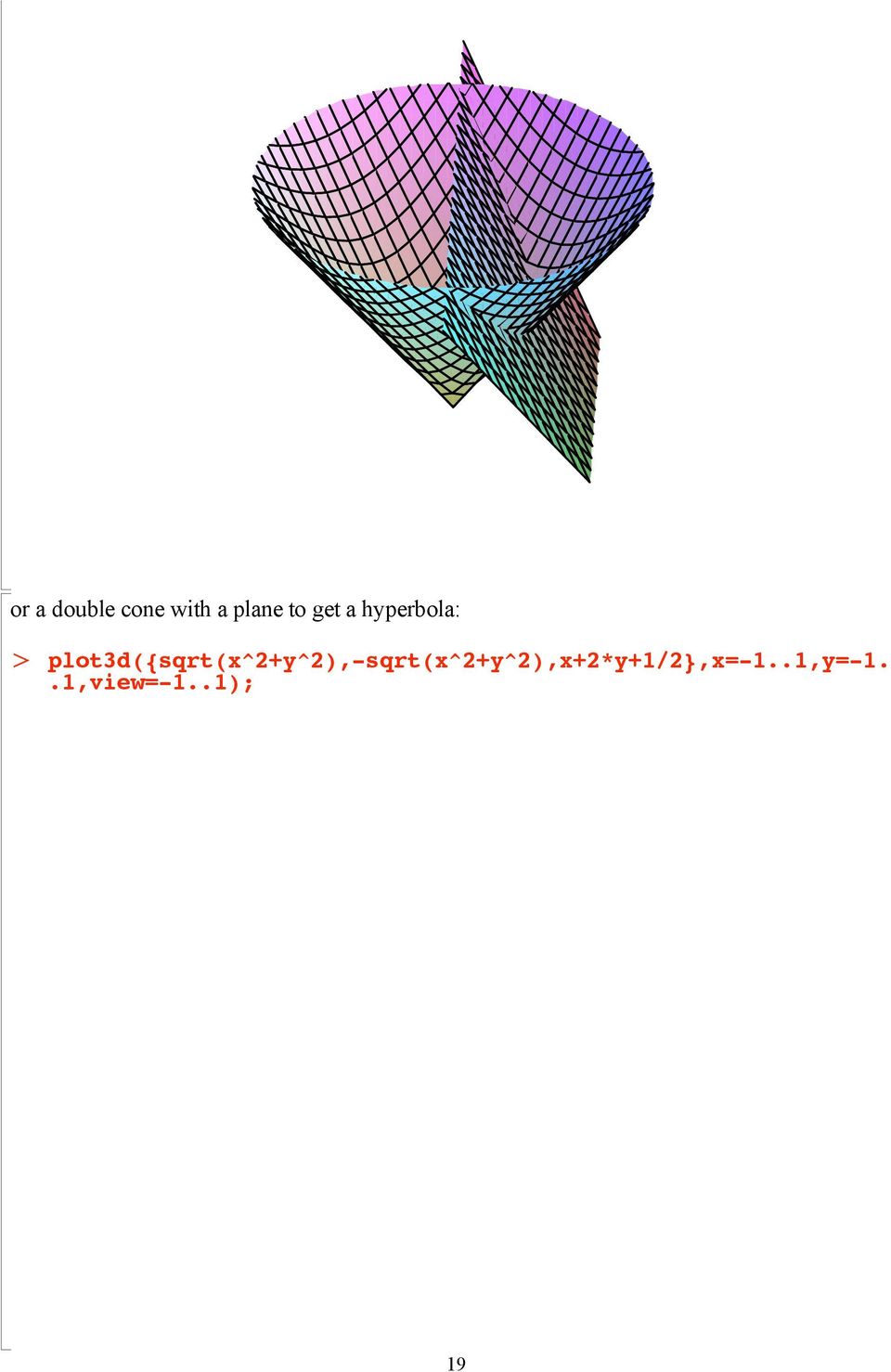
20 or a double cone with a plane to get a hyperbola: plot3d({sqrt(x^2+y^2),-sqrt(x^2+y^2),x+2*y+1/2},x=-1..1,y=-1..1,view=-1..1); 19

21 ne can also plot parametrically, by specifying formulae for the x, y, z coordinates. (This is where you use [ ] brackets.) plot3d([(2+cos(q))*cos(p),(2+cos(q))*sin(p),sin(q)],p=0..2*pi, q=0..2*pi,view=-2..2); a torus 20

22 plot3d([sin(p)*cos(q),sin(p)*sin(q),cos(p)],p=0..pi,q=0..2*pi, view=-1..1); a sphere Three-dimensional Lissajous figures: plot3d([sin(2*p),sin(3*p),cos(5*p)],p=0..2*pi,q=0..1,view=-1..1,numpoints=5000,thickness=3); There are lots of other things you can explore with these functions! plot3d(1.5^x*sin(y),x=-1..2*pi,y=0..pi,coords=spherical); 21

23 Integration The process of integrating is much older than differentiating and goes back to the Ancient Greeks. For example, Archimedes' efforts to measure the area of a circle ( and hence calculate a value for!) in about 250BC are equivalent to trying to integrate a function. Maple will calculate indefinite integrals when it can, but quite "easy" functions may be difficult even for Maple. If you differentiate the integral, you should get back to where you started. int(x^5,x); diff(%,x); f:=int(sqrt(1+sqrt(x)),x); simplify(f); g:=diff(f,x); simplify(g); K 8 15 f := K! K x6 x 5! 1 C x 3/2 3 x K 2! 22

24 8 15 C C x x C C x x K C x g := K K 1 5! 1 C x 3 x K 2 x! K 2 5! 1 C x 3/2 x 1 C x Sometimes Maple can't do it. But it still knows how to get back when it differentiates. f:=int(cos(sqrt(1+x^2)),x); diff(f,x); f := cos 1 C x 2 dx cos 1 C x 2 Sometimes it can do the integral but it isn't much help. int(cos(1+x^3),x); 1 6 cos 1! 9 21/3 2 K 9 7 K x 7 2 2/3 sin x 3 2 2/3 2 7 x6 C 2 sin x 3 3 C 3 2! x 2 LommelS1! x 3 11/6 11 6, 3 2, x3 3 x 7 2 2/3 cos x 3 x 3 K sin x 3 LommelS1! x 3 17/6 2/3 5 6, 1 2, x3 cos x 3 x 3 K sin x 3! x 2 K 1 6 sin 1! 21/3 3 4 K 3 4 C 9 4 x 7 2 2/3 sin x 3 LommelS1! x 3 11/6 x 2 2/3 sin x 3! 5 6, 3 2, x3 K 9 4 x 7 2 2/3 cos x 3 x 3 K sin x 3 LommelS1! x 3 17/6 x 2 2/3 cos x 3 x 3 K sin x , 1 2, x3! Remember, however, that integration should involve a "constant of integration" and so if you integrate a derivative, the answer may look different. 23

25 f:=(1+x^2)^2; g:=diff(f,x); h:=int(g,x); f-h; simplify(f-h); f := 1 C x 2 2 g := 4 1 C x 2 x h := x 4 C 2 x 2 1 C x 2 2 K x 4 K 2 x 2 1 Maple will calculate integrals of trigonometric functions which would be very tedious to tackle "by hand". In every case, differentiation should bring you back to where you started but it might be a bit of a struggle. f:=int(tan(x)^3,x); g:=diff(f,x); simplify(g); f:=sin(x)^3/(1+cos(x)^3); g:=int(f,x); h:=diff(g,x); simplify(h); simplify(h-f); f := 1 2 tan x 2 K 1 2 ln 1 C tan x 2 g := tan x 1 C tan x 2 f := g := 1 2 ln 1 K cos x C cos x 2 K 1 3 h := 1 2 tan x 3 sin x 3 1 C cos x 3 sin x K 2 cos x sin x 1 K cos x C cos x 2 C arctan K tan x 1 C 1 3 sin x K1 C cos x K 1 K cos x C cos x K1 C 2 cos x 3 sin x K1 C 2 cos x Although one can repeatedly integrate a function, there is no shorthand for multiple integration as there is for multiple differentiation. 2 f:=x^2-sin(2*x); int(%,x); 24

26 int(%,x); int(%,x); int(%,x); int(f,x,x,x,x); This only integrates once. f := x 2 K sin 2 x 1 3 x3 C 1 2 cos 2 x 1 12 x4 C 1 4 sin 2 x 1 60 x5 K 1 8 cos 2 x x6 K 1 16 sin 2 x 1 3 x3 C 1 2 cos 2 x Maple will also do definite integrals. It will give an exact answer if it can. Note the way you specify the range of integration: x = etc int(x^4,x=0..1); int(sin(x)^2,x=0..pi); ! The calculation mentioned above that Archimedes used to calculate " (t he quadrature of the circle ) is equivalent to the integral: int(sqrt(1-x^2),x=-1..1); 1 2! Maple will (sometimes) handle integrals over infinite ranges as well as integrals over ranges where the function goes off to infinity. int(exp(-x),x=0..infinity); int(exp(x),x=0..infinity); int(tan(x),x=0..pi/2); int(tan(x),x=0..pi); 1 N N undefined Even if it can't work out exactly what the answer is, you can ask it 25

27 to do a numerical integration by using the evalf function. k:=int(cos(sqrt(1+x^2)),x=0..1); evalf(k); k := 0 1 cos 1 C x 2 dx As in the differentiation case, Maple will write out the formula for the derivative if you ask for (with a capital letter). Int Int(cos(x)^2,x); Int(cos(x)^2,x=0..Pi); evalf(%); Int(cos(x)^5,x)=int(cos(x)^5,x); cos x 2 dx 0! cos x 2 dx cos x 5 dx = 1 5 cos x 4 sin x C 4 15 cos x 2 sin x C 8 15 sin x Solving equations Maple will try and solve equations. You have to give it the equation and tell it what to solve for. If there is only one variable in the equation, it will solve for that without being told. If you give it an expression instead of an equation, it will assume you mean expression = 0. solve(7*x=22,x); solve(7*x=22); solve(7*x-22); solve(all_my_problems); Maple will solve equations which have more than one solution. solve(a*x^2+b*x+c=0,x); solve(x^3-2*x^2-5*x+1=0,x); evalf(%,4); 26

28 1 6 K 1 2 b K 316 C 12 I /3 C C 12 I /3 K C 12 I /3 K K K b 2 K 4 a c a 38, K 1 2 b C b 2 K 4 a c a C 12 I /3 C 2 3, K C 12 I /3 C 2 3 C 1 2 I C 12 I /3, K C 12 I /3 C 2 3 K 1 2 I C 12 I / C 12 I /3 316 C 12 I / K I, K1.576 K I, C I A short cut if you only want to see the decimal expansion is to use the function fsolve. Usually, fsolve will only give the real roots of the equation. There are ways of getting complex roots out of it. If you want to know what they are then you can consult the Help facilities for fsolve. fsolve(x^3-2*x^2-5*x+1=0,x); K , , If you want to find solutions in a particular range you may have to specify it fsolve(sin(x),x=3..4); Maple will solve simultaneous equations. You have to enter the equations as a "set" (with { } round them and commas between). If you want to solve for several variables, you have to enter these as a set too. If you leave out the variables you want to solve for, Maple will assume you want all of them. solve({y=x^2-4,y=-2*x-2},{x,y}); solve({y=x^2-4,y=-2*x-2}); evalf(%); y = K2 Rootf 2 _ZK 2 C _Z 2, label = _L2 K 2, x = Rootf 2 _ZK 2 C _Z 2, label = _L2 y = K2 Rootf 2 _ZK 2 C _Z 2, label = _L4 K 2, x = Rootf 2 _ZK 2 C _Z 2, label = _L4 y = K , x = and of course, you can use fsolve here too. 27

29 fsolve({y=x^2-4,y=-2*x-2},{x,y}); y = K , x = You can then use the plot facility to see the intesection of the two curves. Then you see that we've missed one of the solutions plot({x^2-4,-2*x-2},x=-3..1,colour=black); K3 K2 K1 K1 1 x K2 K3 K4 We can find the missing one by specifying ranges fsolve({y=x^2-4,y=-2*x-2},{x=-3..0,y=0..5}); y = , x = K If there is more than one solution you can pick out the one you want using [1] or [2] or... f:=x^2+3*x+1; sol:=solve(f=0,x); evalf(sol[1]); sol := 1 2 f := x 2 C 3 x C 1 5 K 3 2, K3 2 K 1 2 K and then you can draw the graph to see where it is plot(x^2+3*x+1,x=-1..0); 28

30 1 0.5 K1 K0.8 K0.6 K0.4 K0.2 0 x K0.5 K1 As an illustration of how this can be used, we will calculate the equation of the tangent to a curve = f(x) at some point x 0 say. Recall that if the tangent is y = mx + c the gradient m is the derivative at x = x 0. Then we have to choose the constant c so that the line goes through the point ( x 0, f(x 0 )) y f:=x->sin(x); x0:=0.6; fd:=diff(f(x),x); m:=subs(x=x0,fd); c0:=solve(f(x0)=m*x0+c,c); y=m*x+c0; plot([f(x),m*x+c0],x=0..1,y=0..1,colour=black); f := x/sin x x0 := 0.6 fd := cos x m := cos 0.6 c0 := y = x C

31 1 0.8 y x You could now go back and alter the function f and the point x 0 and run the same bit of code to calculate the equation of the tangent to anything! As a further illustration, we consider the problem of finding a tangent to a circle from a point outside the circle. The circle (well, semi-circle, actually) can be specified by y =!(1+x 2 ) and we'll find a tangent to it from the point (say) (0, 2). We first use the same method as above to calculate the equation of the tangent to the curve at a variable point x 0 We'll begin by unassigning all our variables and then use a similar bit of code to that used above. restart; f:=x->sqrt(1-x^2); fd:=diff(f(x),x); m:=subs(x=x0,fd); c0:=solve(f(x0)=m*x0+c,c); y=m*x+c0; y = K f := x/ 1 K x 2 fd := K m := K c0 := x 1 K x 2 x0 1 K x K x0 2 x0 x C 1 1 K x0 2 1 K x0 2 Then vary x 0 until the tangent goes through the point (0.2). We'll make x 1 the value of x 0 when this happens. Since this produces two answers, we'll choose one of them. 30

32 The gradient m 1 of the tangent is then the value of m at this point and the intercept c 1 on the y-axis is the value of c 0 at this point. So we can find the equation of the tangent: y = m 1 x + c 1. x1:=solve(subs(x=0,y=2,y=m*x+c0),x0)[1]; m1:=subs(x0=x1,m); c1:=subs(x0=x1,c0); y=m1*x+c1; x1 := K m1 := c1 := 4 y = x C 4 We'll plot the answer to see if it really works. plot([f(x),m1*x+c1],x=-2..2,y=-1..2,colour=black); 2 y 1 K2 K x Asking Maple for the second solution above would give another tangent to the circle. K1 You could now replace x = 0, y = 2 by any other point and work out the equation of the tangents going through that point. Looping There are several ways to get Maple to perform what is called a "loop". The first is a for-loop. You put what you want done between the do and the end do. 31

33 Use Shift-Return to get a new line without Maple running the code. for i from 1 to 5 do x:=i; end do; x := 1 x := 2 x := 3 x := 4 x := 5 It is often better to stop Maple printing out everything it does. You can do this by putting a : (a colon) after the loop instead of ; (a semi-colon). Putting a : instead of a ; after any command will stop Maple from printing it out as it executes the command. However, if you do want it to print something about what is going on, you can ask for it with a print command. for i from 1 to 5 do x:=i; print(x); end do: If you want to include some text, you can include it in "back quotes" (between the left-hand shift and the z). Single words (which Maple will interpret as variables) can get away without quotes, but more than one word can't. See below for the effect of the usual ". print(one_word); print(`two words`); print("two words"); one_word two words "two words" print(two words); Error, missing operator or `;` There is another forms of for-loop: one in which we get the variable to increase itself by more than one between implementing the things in the loop: for i from 1 to 15 by 3 do x:=i; 32

34 print(`the value of x is `,x); end do: the value of x is, 1 the value of x is, 4 the value of x is, 7 the value of x is, 10 the value of x is, 13 As an illustration of what to do with a loop, we calculate the sum of an Arithmetic Progression (AP) to several terms e.g. 3, 5, 7, 9,... We will suppress printing in the loop. Suppressing printing has the effect of speeding things up, since it takes Maple much longer to print than to calculate. a:=1;d:=2; term:=a: total:=0: for i from 1 to 100 do total:=total+term; term:=term+d; end do: total; a := 1 d := In a similar way, we can calculate the sum of a Geometric progression (a GP) like 3, 6, 12, 24,... a:=3;r:=2; term:=a: total:=0: for i from 1 to 20 do total:=total+term; term:=term*r; end do: total; a := 3 r := As an illustration of another kind of loop we answer the question of how many terms of a GP we need to take before the sum is > (say) 10000? We use a while-loop which will be implemented until the "boolean expression" in the first line of the loop becomes False. A boolean expression, named after the English mathematician George Boole ( ) who was one of the first to apply mathematial techniques to logic, is something which takes the values either True or False. a:=3; r:=1.1; term:=a:total:=0: 33

35 count:=0: while total < do total:=total+term; term:=term*r; count:=count+1; end do: count; a := 3 r := If clauses We now show how Maple can make a choice of several different things to do. This branching is controlled by soething called an if-clause. We put what we want Maple to do between the then and the end if. Here is an example. a:=90; if a>60 then print(`a is bigger than 60 `);end if; a := 90 a is bigger than 60 In the above, if the boolean expression (between the if and the then) is False, then nothing gets done. We can alter that: a:=50; if a > 60 then print(`a is bigger than 60 `); else print(`a is smaller than 60 `);end if; a := 50 a is smaller than 60 You can put in lots of other alternatives using elif (which stands for else if). a:=50; if a > 60 then print(`a is bigger than 60 `); elif a > 40 then print(`a is bigger than 40 but less than 60 `); else print(`a is smaller than 60 `);end if; a := 50 a is bigger than 40 but less than 60 We can apply these ideas to get Maple to search for the solutions of an equation. For example,consider Pell's equation, named (probably incorrectly) after the English mathematician John Pell (1611 to 1685) but in fact studied by the Indian mathematician Brahmagupta (598 to 660) much earlier. It asks for an integer solution ( a, b) to the equation a 2 K n b 2 = 1 where n is a fixed integer. We'll look for solutions a, b for small(ish) values of a and b. 34

36 n:=5; for a from 1 to 1000 do for b from 1 to 1000 do if a^2-n*b^2=1 then print(a,b); end if; end do;end do: n := 5 9, 4 161, 72 Lists A list in Maple is an ordered set and is written with [ ]. It is often convenient to put results of calculations into such a list. The nth element of a list L (say) can then be referred to later by L[n]. The last element of L is L[-1], etc. You can treat the elements of a list as variables and assign to them. A:=[1,2,3,4,5]; A[3]; A[-2]; A[2..-1]; A[2]:=55; A; A := 1, 2, 3, 4, , 3, 4, 5 A 2 := 55 1, 55, 3, 4, 5 You can't assign to an element that isn't there! A[6]:=22; Error, out of bound assignment to a list The elements of a list are op(a) which stands for the operands of A. To add extra elements: L:=[]; for i from 1 to 100 do L:=[op(L),i^2];end do: L; L := 1, 4, 9, 16, 25, 36, 49, 64, 81, 100, 121, 144, 169, 196, 225, 256, 289, 324, 361, 400, 441, 484, 529, 576, 625, 676, 729, 784, 841, 900, 961, 1024, 1089, 1156, 1225, 1296, 1369, 1444, 1521, 1600, 1681, 1764, 1849, 1936, 2025, 2116, 2209, 2304, 2401, 2500, 2601, 35

37 2704, 2809, 2916, 3025, 3136, 3249, 3364, 3481, 3600, 3721, 3844, 3969, 4096, 4225, 4356, 4489, 4624, 4761, 4900, 5041, 5184, 5329, 5476, 5625, 5776, 5929, 6084, 6241, 6400, 6561, 6724, 6889, 7056, 7225, 7396, 7569, 7744, 7921, 8100, 8281, 8464, 8649, 8836, 9025, 9216, 9409, 9604, 9801, The number of elements in a list is nops ( = number of operands). nops(l); 100 You can delete elements from a list (or replace then) using subsop (= substitute operand). Note that the original list is unchanged. L0:=[1,2,3,4,5]; L1:=subsop(-1=NULL,1=NULL,L0); L2=subsop(1=55,L0); L0; L0 := 1, 2, 3, 4, 5 L1 := 2, 3, 4 L2 = 55, 2, 3, 4, 5 1, 2, 3, 4, 5 As above one can use a for loop to put elements into a list. We could have done the same thing using the seq function: M:=[seq(n^2,n=1..100)]; M := 1, 4, 9, 16, 25, 36, 49, 64, 81, 100, 121, 144, 169, 196, 225, 256, 289, 324, 361, 400, 441, 484, 529, 576, 625, 676, 729, 784, 841, 900, 961, 1024, 1089, 1156, 1225, 1296, 1369, 1444, 1521, 1600, 1681, 1764, 1849, 1936, 2025, 2116, 2209, 2304, 2401, 2500, 2601, 2704, 2809, 2916, 3025, 3136, 3249, 3364, 3481, 3600, 3721, 3844, 3969, 4096, 4225, 4356, 4489, 4624, 4761, 4900, 5041, 5184, 5329, 5476, 5625, 5776, 5929, 6084, 6241, 6400, 6561, 6724, 6889, 7056, 7225, 7396, 7569, 7744, 7921, 8100, 8281, 8464, 8649, 8836, 9025, 9216, 9409, 9604, 9801, restart; You can use $ instead of the seq function (but the variable you use must be unassigned this time). S:=0 $ 5; T:=n^2 $ n=1..10; S := 0, 0, 0, 0, 0 T := 1, 4, 9, 16, 25, 36, 49, 64, 81, 100 The elements of a list do not need to be all the same kind and they can even be other lists: N:=[x^2,[1,2],[]]; 36

38 N := x 2, 1, 2, You can sort lists: sort([1,6,-4,10,5,7]); K4, 1, 5, 6, 7, 10 You can do quite useful things with lists. For example, here are all the primes < The function isprime returns either true or false. L:=[]: for i from 1 to 1000 do if isprime(i) then L:=[op(L),i];end if;end do: L; 2, 3, 5, 7, 11, 13, 17, 19, 23, 29, 31, 37, 41, 43, 47, 53, 59, 61, 67, 71, 73, 79, 83, 89, 97, 101, 103, 107, 109, 113, 127, 131, 137, 139, 149, 151, 157, 163, 167, 173, 179, 181, 191, 193, 197, 199, 211, 223, 227, 229, 233, 239, 241, 251, 257, 263, 269, 271, 277, 281, 283, 293, 307, 311, 313, 317, 331, 337, 347, 349, 353, 359, 367, 373, 379, 383, 389, 397, 401, 409, 419, 421, 431, 433, 439, 443, 449, 457, 461, 463, 467, 479, 487, 491, 499, 503, 509, 521, 523, 541, 547, 557, 563, 569, 571, 577, 587, 593, 599, 601, 607, 613, 617, 619, 631, 641, 643, 647, 653, 659, 661, 673, 677, 683, 691, 701, 709, 719, 727, 733, 739, 743, 751, 757, 761, 769, 773, 787, 797, 809, 811, 821, 823, 827, 829, 839, 853, 857, 859, 863, 877, 881, 883, 887, 907, 911, 919, 929, 937, 941, 947, 953, 967, 971, 977, 983, 991, 997 There are 168 of them! nops(l); 168 Sets Maple can also deal with sets, which it puts in { }. The elements are not in any particular order, and if an element is "repeated" it will be left out. S:={5,3,6,8}; T:={1,2,2,3}; S := 3, 5, 6, 8 T := 1, 2, 3 You can add an element to a set using union: S:=S union {13}; S := 3, 5, 6, 8, 13 You can use other set-theoretic connectives. 37

39 {1,2,3,4} intersect {3,4,5,6}; {1,2,3,4} minus {3,4,5,6}; 3, 4 1, 2 We can get Maple to loop over only certain specified values. We may list these values either as a list: for i in [2,8,5,3] do x:=i; print(`the value of x is `,x); end do: the value of x is, 2 the value of x is, 8 the value of x is, 5 the value of x is, 3 or as a set. If Maple uses a set it will usually put it into order before implementing the commands (but don't count on it). for i in {2,8,5,3} do x:=i; print(`the value of x is `,x); end do: the value of x is, 2 the value of x is, 3 the value of x is, 5 the value of x is, 8 You can find out more with the Help command:?list Summing Earlier we used a for loop to sum the terms of Arithmetic and Geometric Progressions. The process of summing the terms of a sequence is so common that Maple has a special function that lets you do it without writing your own loop. You enter sum(expression, n = a.. b) and Maple will take the sum over the range from a to b. What you sum over had better be an unassigned variable, or there will be trouble. sum(n^2,n=1..100); In fact Maple is clever enough (sometimes) to even work out the general formula for a sum and can (sometimes) sum all the way to infinity. restart; sum(a*r^i,i=1..n); sum(a*r^i,i=1..infinity); 38

40 sum(sin(i),i=1..n); 1 2 sin 1 cos n C 1 cos 1 K 1 a r n C 1 rk 1 K a r rk 1 K a r rk 1 K 1 2 sin n C 1 K 1 2 sin 1 cos 1 cos 1 K 1 C 1 2 sin 1 It knows the answer to the "Basel" problem that Leonhard Euler (1707 to 1783) solved: sum(1/i^2,i=1..infinity); 1 6!2 In the next case it gives the answer in the form of the Riemann zeta function. sum(1/i^3,i=1..infinity); " 3 Sometimes it can't do it. sum(cos(sqrt(n)*pi),n=1..n); sum(cos(sqrt(n)*pi),n=1..10); evalf(%); N >n = 1 cos n! K1 C cos 2! C cos! 3 C cos 5! C cos 6! C cos 7! C cos 8! C cos 10! K Maple knows what happens if "something goes wrong" sum(i*(-1)^i,i=1..100); sum(i*(-1)^i,i=1..infinity); 50 N >i = 1 i K1 i As with Diff and Int using a capital letter just prints the formula: Sum(i*(-1)^i,i=1..100); evalf(%); 100 >i = 1 i K1 i

41 Procedures We saw earlier how to define a function using an assignment like: f := x -> x^2; This is in fact shorthand for using a construction known as a procedure. We can get the same effect with: f:=proc(x) x^2; end proc; f(20); f := proc x x^2 end proc 400 Procedures can act like functions and return a value (like x 2 in the above example) but can implement functions which are more complicated than just evaluating a formula. For example, we can adapt the code we wrote above to define a procedure which returns the number of terms of a Geometric Progression needs for its sum to go past some given value n. Note that variables which are only needed inside the procedure get declared to be local, so that if the same variable names had been used somewhere else, these will not be changed by the procedure. howmanyterms:=proc(x) local term,total,count; term:=a:total:=0: count:=0: while total<x do total:=total+term; term:=term*r; count:=count+1; end do: count; end proc; howmanyterms := proc x local term, total, count; term := a; total := 0; count := 0; while total! x do total := total C term; term := term* r; count := 1 C count end do; count end proc The value returned by the procedure is the last thing in the listing before the end statement. If we had wished we could have put return count; as the last thing in the "body of the procedure". Notice that Maple will pretty-print the procedure, indenting the code to indicate where the procedure or loops start and finish. To call the procedure, we tell Maple what the values of a and r are and then apply the procedure to a number. a:=3;r:=2; howmanyterms(10000); a := 3 40

42 r := 2 12 We can use an if-clause to define a function. f:=proc(x) if x < 0 then x^2; else x+1; end if;end proc; f(-1); f(3); f := proc x if x! 0 then x^2 else x C 1 end if end proc 1 4 We can plot this function, but it is necessary to be a bit careful plotting functions defined by procedures, otherwise Maple gets unhappy. You can either plot them without mentioning the variables at all, by: plot( f, ); or you can do it by putting in some single quotes: ' ': plot('f(x)', x = -1..1); If the variable x had been assigned to you would have to put that in quotes too. plot(f,-1..1); K1 K We count the primes up to a real number n. When we plot this we get a kind of "step function". countprimes:=proc(n) local count,i; count:=0; for i from 1 to n do if isprime(i) then count:=count+1;end if; end do; return count; end proc; countprimes := proc n local count, i; count := 0; for i to n do if isprime i return count end proc then count := count C 1 end if end do; 41

43 plot(countprimes,1..100); plot(countprimes, ); There is a "flat bit" near 890. In fact a sequence of 19 consecutive non-primes from 888 to 906. plot(countprimes, ); The French mathematician Adrien-Marie Legendre (1752 to 1833) approximated the growth of the number of primes with the function: L:=x/(log(x)-1.08); L := x ln x K

44 plot(['countprimes(x)',l],x=0..100,0..25,colour=[black,red]); x The German mathematician Carl Friedrich Gauss (1777 to 1855) used a different approximation: the logarithmic integral: logint:=proc(x) return int(1/log(t),t=2..x); end proc; logint := proc x return int 1 / log t, t = 2..x end proc plot([countprimes,logint],1..100,colour=[black,red]); You can see these different approximations together(we'll specify the colours since otherwise Maple will use colours which do not print well): plot(['countprimes(x)',l,'logint(x)'],x=0..100,0..25,colour= [black,red,blue]); 43

45 x More Procedures If you want to make a procedure do something to a variable you have already defined outside the procedure, you have to declare it as global. We'll add an element to the end of a list. In this case we don't want to return anything so we put return; and nothing else at the end of the procedure. addon:=proc(x) global A; A:=[op(A),x]; return; end proc; Then apply this: addon := proc x global A; A := op A, x ; return end proc A:=[1,2,3]; addon(0); A; A := 1, 2, 3 1, 2, 3, 0 We could do something similar without using a global variable. But notice that in this case the original list is unchanged. addend:=proc(a,x) return [op(a),x]; end proc; addend := proc A, x return op A, x end proc A:=[1,2,3]; B:=addend(A,0); A; A := 1, 2, 3 44

46 B := 1, 2, 3, 0 1, 2, 3 ne thing to be careful of is that you cannot assign to the parameters passed to the procedure as if they were local variables. test:=proc(n) n:=n+1; return n end proc; test := proc n n := n C 1; return n end proc test(9); Error, (in test) illegal use of a formal parameter Reversing As an example of the use of procedures we'll use Maple to find a solution to the following problem: Find a four digit number which is multiplied by 4 when its digits are reversed. We start by defining a procedure which turns the digits of a number into a list. Note that we test each procedure as we write it. digits:=proc(n) local ans,m,d; m:=n;ans:=[]; while m<>0 do d:=m mod 10;m:=(m-d)/10;ans:=[d,op(ans)]; end do; return ans; end proc; digits := proc n local ans, m, d; m := n; ans := ; while m!0 do d := mod m, 10 ; m := 1 / 10 * m K 1 / 10 * d; ans := end do; return ans end proc K:=digits( ); K := 1, 2, 3, 4, 5, 0, 0, 8 d, op ans It's easy to write a list in the opposite order: reverselist:=proc(l) local i,m; M:=[]; 45

47 for i from 1 to nops(l) do M:=[L[i],op(M)]; end do; return M; end proc; reverselist := proc L local i, M; M := ; for i to nops L do M := L i, op M end do; return M end proc reverselist(k); 8, 0, 0, 5, 4, 3, 2, 1 Now we have to get a number back from its list of digits buildit:=proc(l) local ans,i; ans:=0; for i from 1 to nops(l) do ans:=10*ans+l[i]; end do; return ans; end proc; buildit := proc L local ans, i; ans := 0; for i to nops L do ans := 10 * ansc L i end do; return ans end proc buildit(k); Put the ingredients together: reversenum:=proc(n) buildit(reverselist(digits(n))); end proc; reversenum := proc n buildit reverselist digits n end proc reversenum(78531); Now we can look for our four digit number for n from 1000 to 9999 do if reversenum(n)=4*n then print(n); end if end do: 2178 Do the same for a 5 digit number for n from to do 46

48 if reversenum(n)=4*n then print(n); end if end do: and even for a 6 digit number for n from to do if reversenum(n)=4*n then print(n); end if end do: So it looks as if we might have a theorem! *4; An old question asks if one can always make a number "palindromic" by adding it to its reverse n:=1790; count:=0: while reversenum(n)<>n do n:=n+reversenum(n); print(n); count:=count+1; end do: print(`palindromic in `,count,` steps`); n := Palindromic in, 3, steps Numbers to try are 89 or 296 or.... A number NT to try is 196 n:=196; count:=0: while reversenum(n)<>n do n:=n+reversenum(n); print(n); count:=count+1; end do: print(`palindromic in `,count,` steps`); n := Warning, computation interrupted 47

49 Pythagorean triples We can use Maple to search for solutions to equations with integer solutions. Such equations are called Diophantine after the Greek mathematician Diophantus of Alexandria (200 to 284 AD). For example, looking for Pythagorean triples satisfying a 2 C b 2 = c 2 we can use the Maple function type(x, integer) to check whether a number has an integer square root. We take y # x since otherwise we will get each pair ( x, y) twice. for x from 1 to 20 do for y from x to 20 do if type(sqrt(x^2+y^2),integer) then print(x,y,sqrt(x^2+y^2)) fi; od od: 3, 4, 5 5, 12, 13 6, 8, 10 8, 15, 17 9, 12, 15 12, 16, 20 15, 20, 25 Here are all solutions up to x = 100 and y = 100. We'll leave out those which are multiples of others we have found. We do this by insisting that x and y have no factor bigger than 1 in common. We arrange this using the igcd (= integer greatest common divisor or highest common factor) function. Notice how we combine the two conditions with an and. L:=[]: for x from 1 to 100 do for y from x to 100 do if type(sqrt(x^2+y^2),integer) and igcd(x,y) = 1 then L:=[op(L),[x,y,sqrt(x^2+y^2)]]; fi; od: od: L; 3, 4, 5, 5, 12, 13, 7, 24, 25, 8, 15, 17, 9, 40, 41, 11, 60, 61, 12, 35, 37, 13, 84, 85, 16, 63, 65, 20, 21, 29, 20, 99, 101, 28, 45, 53, 33, 56, 65, 36, 77, 85, 39, 80, 89, 48, 55, 73, 60, 91, 109, 65, 72, 97 Some other equations Similarly, we can look for non-zero solutions of other equations like a 2 C 2 b 2 = c 2 or 2 a 2 C 3 b 2 = c 2 or... Sometimes we don't find any and then we could try and prove mathematically that no such solution exists! 48

50 for a from 1 to 100 do for b from 1 to 100 do c:=sqrt(2*a^2+3*b^2); if type(c,integer) then print(a,b,c); end if; end do end do: Work modulo 3 to see that one can't find solutions to this last one! We can now look again at Pell's equation, and solve it more efficiently than we did before. We look for a solution (x, y) to the equation n x 2 C 1 = y 2 where n is a fixed integer. n:=2: for x from 0 to 2000 do y:=sqrt(n*x^2+1); if type(y,integer) then print(x,y); end if; end do: 0, 1 2, 3 12, 17 70, , 577 Can you see what recurrence relation is satisfied by the solution? If you could you could generate lots more solutions. n:=5: for x from 0 to 2000 do y:=sqrt(n*x^2+1); if type(y,integer) then print(x,y); end if; end do: 0, 1 4, 9 72, , 2889 It's harder to spot the relation this time. Though if you take the clue from the last one you might manage it! The next pair is: (23184, 51841) 51841^2-5*23184^2; 1 The Indian mathematician Brahmagupta solved the equation in 628AD with n = 83 and found solutions: (9, 82), (1476, 13447), (242055, ), ( , ), ( , ), ( , ), ( , ) Interpolation A parabola has an equation y = a x 2 C b x C c with three coefficients we can choose. So in general one can find a (unique!) parabola through any three points in the plane. We'll call the points p, q, r and each point will be a list of length 2. 49

51 restart; parab:=proc(p,q,r) local par,a,b,c,eqn1,eqn2,eqn3,s; par:=a*x^2+b*x+c; eqn1:=subs(x=p[1],p[2]=par); eqn2:=subs(x=q[1],q[2]=par); eqn3:=subs(x=r[1],r[2]=par); s:=solve({eqn1,eqn2,eqn3},{a,b,c}); subs(s,par); end proc; parab := proc p, q, r local par, a, b, c, eqn1, eqn2, eqn3, s; par := a * x^2 C b * x C c; eqn1 := subs x = p 1, p 2 = par ; eqn2 := subs x = q 1, q 2 = par ; eqn3 := subs x = r 1, r 2 = par ; s := solve eqn1, eqn2, eqn3, a, b, c ; subs s, par end proc parab([-1,-4],[2,-1],[1,3]); K 5 2 x2 C 7 2 x C 2 We'll now plot the parabola and some points. We do this by assigning our plots (things Maple calls "Plot structures" to variables P and Q and then using the display function from the plots package. Note how we plot the individual points. You can use?plot[options] to see what all the other things you can specify are. points:=[-1,-1],[2,-2],[1,2]; P:=plot(parab(points),x=-2..3,-3..3): Q:=plot({points},style=point,symbol=cross,symbolsize=20, colour=blue): plots[display]([p,q]); points := K1, K1, 2, K2, 1, K2 K K1 x K2 K3 50

52 More plotting You can use a similar method to animate the drawing of (for example) curves. Put all the curves (one "frame" at a time) into a list and then give it to plots[display]. If you want to see the result with the frames in sequence put in insequence=true otherwise you'll get them all on top of one another. Then click on the window and choose Play from the Animation window or click on the Play icon on the tool bar. The only problem with this is that it can produce very large files. restart; L:=[]: for k from 0 to 10 by 0.2 do L:=[op(L),plot(cos(k*sin(x)),x=0..Pi,-1..1)]; end do: plots[display](l,insequence=true); K x K1 In polar coordinates: L:=[]: for k from 0.1 to 10 by 0.1 do L:=[op(L),plot([(t/5),t,t=0..k*Pi],coords=polar,thickness=2)] ; end do: plots[display](l,insequence=true); 2 1 K3 K2 K K1 L:=[]: 51 K2

53 for k from 0 to 20 by 0.5 do L:=[op(L),plot([sin(k*cos(t)),t,t=0..2*Pi],coords=polar)]; end do: plots[display](l,insequence=true); K0.8 K0.6 K0.4 K K0.5 You can also animate 3-dimensional pictures in a similar way. If you do a lot of this, there are commands plots[animate] and plots[animate3d] which you can learn about. K1 L:=[]: for k from -1 to 1 by 0.01 do L:=[op(L),plot3d(k*(x^2+y^2),x=-1..1,y=-1..1,view=-1..1)]; end do: plots[display](l,insequence=true); L:=[]: for k from 0 to 3 by 0.1 do 52

54 L:=[op(L),plot3d([sin(p)*cos(q),sin(p)*sin(q),p^k],p=0..Pi,q= 0..2*Pi)]; end do: plots[display](l,insequence=true); Recursion restart; Maple will let procedures call themselves. This is called recursion. f course they can't carry on doing this indefinitely, so things have always got to be arranged so that the process terminates. ne of the best known illustrations is the process by which the Fibonnaci numbers: 1, 1, 2, 3, 5, 8, 13, 21,... are calculated. These were introduced by Fibonacci of Pisa (1170 to 1250) who was the person who introduced the Arabic (or Indian) numeral system to Europe. He introduced them in a problem involving rabbit breeding, but in fact they were known by the Indian mathematician Hemchandra more than 50 years earlier (and other Indians had considered them even before that). fib:=proc(n) if n<3 then 1;else fib(n-1)+fib(n-2);end if;end proc; fib := proc n if n! 3 then 1 else fib n K 1 C fib n K 2 end if end proc fib(35);

55 Unfortunately the process by which this works is "exponential" in n and so it is not a very practical algorithm. We can see how the time increases by modifying our program. fib:=proc(n) global count; count:=count+1; if n<3 then 1;else fib(n-1)+fib(n-2);end if; end proc; fib := proc n global count; count := count C 1; if n! 3 then 1 else fib n K 1 C fib n K 2 end proc count:=0:start:=time(): fib(30); print(count,` calls `,time()-start,` secs`); , calls, 5.698, secs count:=0:start:=time(): fib(35); print(count,` calls `,time()-start,` secs`); end if , calls, , secs To get round this, Maple has a device: option remember; which stores the result of any calculation so it doesn't have to do it again. This makes the calculation linear in n. fib0:=proc(n) option remember; global count; count:=count+1; if n<3 then 1;else fib0(n-1)+fib0(n-2);end if; end proc; fib0 := proc n option remember; global count; count := count C 1; if n! 3 then 1 else fib0 n K 1 C fib0 n K 2 end proc count:=0:start:=time(): fib0(300); print(count,` calls `,time()-start,` secs`); end if , calls, 0.003, secs 54

56 We can apply a similar process to calculating the elements of Pascal's triangle. bc:=proc(n,r) if r>n then 0; elif r=0 then 1 else bc(n-1,r-1)+bc(n-1,r);end if; end proc; bc := proc n, r if n! r then 0 elif r = 0 then 1 else bc n K 1, r K 1 C bc n K 1, r end proc end if Unfortunately this too soon gets out of control! bc(30,13); Warning, computation interrupted To see why: bc:=proc(n,r) global count; count:=count+1; if r>n then 0; elif r=0 then 1 else bc(n-1,r-1)+bc(n-1,r);end if; end proc; bc := proc n, r global count; count := count C 1; if n! r then 0 elif r = 0 then 1 else bc n K 1, r K 1 C bc n K 1, r end proc count:=0:start:=time(): bc(20,10); print(count,` calls `,time()-start,` secs`); , calls, 3.057, secs count:=0:start:=time(): bc(25,10); print(count,` calls `,time()-start,` secs`); end if , calls, , secs Again option remember; gets us out of the hole! bc0:=proc(n,r) option remember; global count; count:=count+1; if r>n then 0; elif r=0 then 1 else bc0(n-1,r-1)+bc0(n-1,r); end if; end proc; 55

57 bc0 := proc n, r option remember; global count; count := count C 1; if n! r then 0 elif r = 0 then 1 else bc0 n K 1, r K 1 C bc0 n K 1, r end proc count:=0:start:=time(): bc0(20,10); print(count,` calls `,time()-start,` secs`); end if More recursion , calls, 0.001, secs The highest common factor or greatest common divisor can be defined very economically using a recursive procedure. This already exists as a standard Maple function igcd. hcf:=proc(a,b) if b mod a =0 then a else hcf(b mod a,a);end if;end proc; hcf := proc a, b if mod b, a = 0 then a else hcf mod b, a, a end if end proc hcf(12345,7896); igcd(12345,7896); 3 3 ne can also implement the Euclidean algorithm which writes the hcf as a combination of the original numbers. You can get this as a standard Maple function as igcdex (= extended integer gcd ). euclid:=proc(a,b) local t; if b mod a=0 then return a,1,0; else t:=euclid(b mod a,a); return t[1],t[3]-t[2]*(trunc(b/a)),t[2]; end if; end proc; euclid := proc a, b local t; if mod b, a = 0 then return a, 1, 0 else t := euclid mod b, a, a ; return t 1, t 3 K t 2 * trunc b / a, t 2 56

58 end if end proc euclid(12345,7896); 3, K197, 308 igcdex(12345,7896,'s','t');s;t; 3 Looking for prime numbers K Recall that a prime number is an integer which is not exactly divisible by any smaller integer except ±1. Maple tests for primeness using the function isprime which returns the answer True or False. For example, we may look for the next prime after (say) (Actually, Maple has a function nextprime which would do this for us, but let's not spoil the fun.) a:= ; while not isprime(a) do a:=a+1;end do: a; a := We may count the number of primes in any given range. The German mathematician Gauss ( ) was interested in how the primes were distributed and when he had any free time, he would spent 15 minutes calculating the primes in a "chiliad" ( a range of a 1000 numbers). By the end of his life, it is reckoned that he had counted all the primes up to about two million. countprimes:=proc(n) option remember; local count,i; count:=0: for i from n* to n* by 2 do if isprime(i) then count:=count+1;fi; end do: count; end proc; countprimes := proc n option remember; local count, i; count := 0; for i from 1000 * n C 1 by 2 to 1000 * n C 1000 do end do; if isprime i then count := count C 1 end if 57

59 count end proc plot('countprimes(round(x))',x=0..100); x There are some other interesting places to look for primes. The mathematician Leonhard Euler ( ) discovered that the formula x 2 K x C 41 is particularly prime-rich. In fact it produces primes for every integer from 1 to 40 (but not, of course, for x = 41) and for lots of others as well. howmanyprimes:=proc(n) local count,x; count:=0: for x from 1 to n do if isprime(x^2-x+41) then count:=count+1;end if; end do: count; end proc; howmanyprimes(40); howmanyprimes(400); howmanyprimes := proc n local count, x; count := 0; for x to n do if isprime x^2 K x C 41 count end proc then count := count C 1 end if end do;

60 For many years mathematicians have tried to find big primes. The French mathematician Fermat ( ) best known for his so-called Last Theorem, investigated primes in the sequence 2 n + 1. for n from 1 to 50 do if isprime(2^n+1) then print(n,2^n+1); end if;end do: 1, 3 2, 5 4, 17 8, , You should note that the values of n which give primes are all of the form 2 m, but that n = 32 does not give a prime. Euler was the first to show (150 years after Fermat guessed that would be prime) that it is composite. You can use the Maple function ifactor (= integer factorise) to verify this. (In fact nobody knows if the formula 2 2m +1 produces any other primes after m = 4, though a lot of effort has gone into looking for them.) a:=2^32+1; ifactor(a); a := ne of Fermat's correspondents was the mathematician Mersenne ( ). He too investigated primes and looked at numbers of the form 2 n 1. for n from 1 to 150 do m:=2^n-1; if isprime(m) then print(n,m);end if; end do: 2, 3 3, 7 5, 31 7, , , , , , ,

61 107, , In fact it is fairly easy to show that if n is not prime the neither is 2 n 1. For example, is divisible by and by (2^35-1)/(2^5-1);(2^35-1)/(2^7-1); Prime numbers of the form 2 n K 1 are called Mersenne primes and they are almost always the largest primes known. This is because a French mathematician called Lucas ( ) invented a test for such primes using the Fibonacci numbers. In 1876 he proved that the number K 1 (see above) is prime. This was the largest known prime until people started using computers in the 1950's. At present 46 Mersenne primes are known. The most recent is K 1 and was discovered on 6th September 2008 using GIMPS (the Great InterNet Mersenne Prime Search). The largest (and largest known prime) was the 45th to be discovered and was found on August 23rd 2008 and is K 1. With a bit of effort, we can show that it has decimal digits (and won a prize of $ for being the first one found with more than 10 million digits). evalf( *log[10](2)); This is (well) outside the range of Maple, but you can test the next after those listed above. isprime(2^521-1); true Testing for primes The Maple function isprime uses an indirect method for deciding whether or not a number is probably prime. It is based on a Number Theory result called Fermats Little Theorem: If p is prime then for any a we have a p = a modulo p. In particular, if one can find a number a for which the above does not hold, then p is not prime. If the above holds with a = 2, 3, 7 then we'll call p a probprime. Note that to run a test like this we need to be able to work out high powers efficiently. Maple has some tricks for doing this. First: how not to do it: To calculate (say) modulo you can get Maple to calculate this (very) big number and then reduce it modulo p:= ; 60

62 n:=2^p: n mod p; p := Much more efficiently, it can reduce modulo p as it goes along and never have to handle integers bigger than p. To do this use &^ instead of ^. p:= ; 2&^p mod p; p := So we'll test a prime candidate with some a: testa:=proc(n,a) a&^n mod n=a;end proc; testa( ,2); testa := proc n, a mod a &^ n, n = a end proc 2 = 2 probprime:=proc(n) testa(n,2) and testa(n,3) and testa(n,5) and testa(n,7); end proc; probprime := proc n testa n, 2 and testa n, 3 and testa n, 5 and testa n, 7 end proc probprime( ); true Let's see how good out test is by comparing it with the isprime function in Maple.. for n from 3 to 2000 by 2 do if probprime(n) and not isprime(n) then print(n); end if; end do: In fact, the above numbers will pass testa for any value of a. They are called Carmichael numbers or pseudoprimes. The isprime test in Maple uses a (slightly) more sophisticated test. It is not known to produce any incorrect answers! The Linear Algebra package 61

63 A lot of clever stuff has been written for Maple and has been put into Packages. To see what packages are available type in?index,package. restart; The LinearAlgebra package lets you work with Matrices (and Vectors). Note that all the commands in this package have capital letters. with(linearalgebra); &x, Add, Adjoint, BackwardSubstitute, BandMatrix, Basis, BezoutMatrix, BidiagonalForm, BilinearForm, CharacteristicMatrix, CharacteristicPolynomial, Column, ColumnDimension, Columnperation, ColumnSpace, CompanionMatrix, ConditionNumber, ConstantMatrix, ConstantVector, Copy, CreatePermutation, CrossProduct, DeleteColumn, DeleteRow, Determinant, Diagonal, DiagonalMatrix, Dimension, Dimensions, DotProduct, EigenConditionNumbers, Eigenvalues, Eigenvectors, Equal, ForwardSubstitute, FrobeniusForm, GaussianElimination, GenerateEquations, GenerateMatrix, GetResultDataType, GetResultShape, GivensRotationMatrix, GramSchmidt, HankelMatrix, HermiteForm, HermitianTranspose, HessenbergForm, HilbertMatrix, HouseholderMatrix, IdentityMatrix, IntersectionBasis, IsDefinite, Isrthogonal, IsSimilar, IsUnitary, JordanBlockMatrix, JordanForm, LA_Main, LUDecomposition, LeastSquares, LinearSolve, Map, Map2, MatrixAdd, MatrixExponential, MatrixFunction, MatrixInverse, MatrixMatrixMultiply, MatrixNorm, MatrixPower, MatrixScalarMultiply, MatrixVectorMultiply, MinimalPolynomial, Minor, Modular, Multiply, NoUserValue, Norm, Normalize, NullSpace, uterproductmatrix, Permanent, Pivot, PopovForm, QRDecomposition, RandomMatrix, RandomVector, Rank, RationalCanonicalForm, ReducedRowEchelonForm, Row, RowDimension, Rowperation, RowSpace, ScalarMatrix, ScalarMultiply, ScalarVector, SchurForm, SingularValues, SmithForm, SubMatrix, SubVector, SumBasis, SylvesterMatrix, ToeplitzMatrix, Trace, Transpose, TridiagonalForm, UnitVector, VandermondeMatrix, VectorAdd, VectorAngle, VectorMatrixMultiply, VectorNorm, VectorScalarMultiply, ZeroMatrix, ZeroVector, Zip The above lets you use all the functions it lists. If you don't want to see this list, put : instead of ; when you enter with (... ). If you ever use restart; you will have to read the package in again. 62

64 A matrix is a "box of numbers". There are several ways to enter matrices. You tell Maple the number of rows and columns (or just how many rows if you want a square one). (In fact you don't need to read the package for this bit.) The second parameter is a list of lists. Maple will put in 0 if you don't tell it what the entry is. A:=Matrix(2,[[a,b],[c,d]]); B:=Matrix(2,3,[[a,b,c],[d,e,f]]); C:=Matrix(3,2,[[a,b],[c]]); Z:=Matrix(2,1); A := a b c d B := C := a b c d e f a b c Z := 0 0 You can enter a matrix by rows: written < a b c > or by columns: < a, b, c > and then rows of columns or columns of rows. There is something called the matrix palette on the View menu which can help, A:=<<a b c>,<d e f>,<g h i>>; B:=<<a,b,c> <d,e,f> <g,h,i>>; a b c A := d e f g h i B := a d g b e h c f i You can initialise the entries of a matrix using a double for-loop or you can use the following: M := Matrix(3,5,(i,j) -> i+2*j); M :=

65 You can even get a matrix with "unassigned variables" for all the entries. M := Matrix(3,(i, j) -> m[i,j]); m 1, 1 m 1, 2 m 1, 3 M := m 2, 1 m 2, 2 m 2, 3 m 3, 1 m 3, 2 m 3, 3 You can add or subtract matrices of the same size and can multiply them by a number (or a variable) using *. A:=<<a b>,<c d>>; B:=<<e f>,<g h>>; C:=<<p q>,<r s>>; A+B; A-B; 3*C; A := a b c d B := e f g h C := p q r s a C e b C f c C g d C h a K e b K f c K g d K h 3 p 3 q 3 r 3 s You can multiply together matrices of compatible shapes by A.B; and you can take powers of matrices by (for example) A^3; or A^(-1); (giving the inverse of the matrix). A.B;A^3;A^(-1); a e C b g a f C b h c e C d g c f C d h a 2 C b c a C a b C b d c a 2 C b c b C a b C b d d c a C d c a C b c C d 2 c c a C d c b C b c C d 2 d 64

66 d a d K b c K c a d K b c K b a d K b c a a d K b c Multiplication of square matrices is associative: A.(B.C) = (A.B).C and distributive A.(B + C) = A.B + A.C but not (in general) commutative A.B $ B.A. (A.B).C-A.(B.C); a e C b g p C a f C b h rk a e p C f r K b g p C h r, a e C b g q C a f C b h sk a e q C f s K b g q C h s, c e C d g p C c f C d h rk c e p C f r K d g p C h r, c e C d g q C c f C d h sk c e q C f s K d g q C h s simplify(%); A.(B+C)-(A.B+A.C); a e C p C b g C r K a e K b g K a p K b r, a f C q C b h C s K a f K b h K a q K b s, c e C p C d g C r K c e K d g K c p K d r, c f C q C d h C s K c f K d h K c q K d s simplify(%); A.B-B.A; b g K c f a f C b h K e b K f d c e C d g K g a K h c c f K b g simplify(%); b g K c f a f C b h K e b K f d c e C d g K g a K h c c f K b g Here are some useful matrices: RandomMatrix produces a matrix with entries in the range IdentityMatrix(4); ZeroMatrix(2,3); RandomMatrix(3,2); 65

67 K50 K79 30 K The determinant of a matrix is a combination of the entries of a square matrix (in rather a complicated way!) which has the property that it is 0 if the matrix does not have an inverse. N:=<<a b>,<c d>>; Determinant(N); N := a b c d a d K b c Determinant(M); m 1, 1 m 2, 2 m 3, 3 K m 1, 1 m 2, 3 m 3, 2 C m 2, 1 m 3, 2 m 1, 3 K m 2, 1 m 1, 2 m 3, 3 C m 3, 1 m 1, 2 m 2, 3 K m 3, 1 m 2, 2 m 1, 3 We can use Maple to demonstrate a theorem discovered by the English mathematician Cayley and the Irish mathematician William Hamilton. Arthur First we take a "general matrix". n:=2; A:=Matrix(n,(i,j)->a[i,j]); n := 2 A := a 1, 1 a 1, 2 a 2, 1 a 2, 2 Id:=IdentityMatrix(n); Id := Then we take the determinant of the matrix A - xi where x is an unassigned variable. This is a polynomial in x called the characteristic polynomial. 66

68 (The roots (possibly complex!) of this are the eigenvalues.) Then the Cayley-Hamilton theorem says that the matrix A satisfies its characteristic polynomial. That is, if we substitute A for x in this polynomial, we get the zero matrix. p:=determinant(a-x*id); p := a 1, 1 a 2, 2 K a 1, 1 x K x a 2, 2 C x 2 K a 1, 2 a 2, 1 p:=collect(p,x); p := x 2 C Ka 1, 1 K a 2, 2 x C a 1, 1 a 2, 2 K a 1, 2 a 2, 1 Unfortunately, Maple won't let you use the subs function with matrices so we do it the hard way. Q:=sum(coeff(p,x,k)*A^k,k=0..n); Q := a 1, 1 a 2, 2 K a 1, 2 a 2, 1 C Ka 1, 1 K a 2, 2 a 1, 1 a 1, 2 a 2, 1 a 2, 2 C a 1, 1 a 1, 2 a 2, 1 a 2, 2 2 simplify(q); Changing n from 2 to a bigger number will make Maple do more work but the result still holds! The Power method As an example of how to use the LinearAlgebra package we'll look at a technique for calculating the largest eigenvalue of a linear transformation. We use the fact that if we apply the transformation over and over again to a vector the resulting vectors settle down to being in the same line and this is the direction of an eigenvector (associated with the largest eigenvalue). In fact this method works providing the largest (in absolute value) eigenvalue is real and distinct. restart; with(linearalgebra): A:=Matrix(2,[[2,1],[3,-4]]); A := K4 It doesn't matter what vector we start at. V:=Vector([-2,1]); V := K2 1 67

69 We'll print the vector and also something that enables us to see its direction. for n from 1 to 15 do W:=(A^n).V; print(w,evalf(w/norm(w,2),5)); end do: K3 K10, K K K16 31, K K1 K172, K K K , K K3262, K K , K K64000, K K , K K , K K , K K , K K , K K , K

70 K , K K , K After a few steps the vectors are "settling down". We can now calculate how the vectors are stretched each time: the eigenvalue : evalf((a.w)[1]/w[1]); K Maple will calculate the eigenvalues and associated eigenvectors. E:=evalf(Eigenvectors(A)); E := K , K We've got quite close to the larger eigenvalue. To see how good our estimate of the eigenvector is: ev:=column(e[2],2); ev/norm(ev,2); ev := K K So it wasn't bad. We can do the same thing with more iterations (and a different starting vector!): A:=Matrix(2,[[2,1],[3,-4]]); V:=Vector([-2,0.9]); W:=(A^100).V: W/Norm(W,2); evalf((a.w)[1]/w[1]); A := K4 V := K2 0.9 K K

71 This process will only settle down if there is a real dominating eigenvalue. For example: A:=Matrix(2,[[1,3],[-3,1]]); V:=Vector([-1,1]); for n from 1 to 10 do W:=(A^n).V; print(w,evalf(w/norm(w,2),5)); end do: 1 3 A := K3 1 V := K , K2, K K44, K K124 K68, K K K , K , K464, K K13808, K K38368 K22976, K K K , K

72 It never settles down since the eigenvalues are complex: E:=evalf(Eigenvectors(A)); 1. C 3. I E := 1. K 3. I, K1. I 1. I Using dsolve restart; We explore the dsolve Maple function. First we define a differential equation. We can use a variety of notations. Note the form of the second derivative using the D notation. We'll look at the equation of (say) a pendulum executing SHM with a damping term a. deq:=diff(x(t),t$2)+a*diff(x(t),t)+x(t)=0; deq := d2 dt 2 x t C a d dt x t C x t = 0 deq:=d(d(x))(t)+a*d(x)(t)+x(t)=0; deq := D 2 x t C a D x t C x t = 0 deq:=(d@@2)(x)(t)+a*d(x)(t)+x(t)=0; deq := D 2 x t C a D x t C x t = 0 dsolve(deq,x(t)); x t = _C1 e K1 2 a C 1 2 a 2 K 4 t C _C2 e K 1 2 a K 1 2 a 2 K 4 t This general solution contains "arbitrary constants". We can get rid of them by specifying boundary or initial conditions. To specify the derivative we must use the D notation. s:=dsolve({deq,x(0)=p,d(x)(0)=q},x(t)); s := x t = 1 2 a p C a 2 K 4 p C 2 q e K1 2 a C 1 2 a 2 K 4 a 2 K 4 t K q C a p K a 2 K 4 p e K1 2 a K 1 2 a 2 K 4 a 2 K 4 t We get different kinds of solution for a < 0 (negative damping), a = 0 (undamped), 0 < a < 2 (light damping), a = 2 (critical damping) and a > 2 (heavy damping). For example: 71

73 CRITICAL DAMPING (This is how a measuring instrument is damped so that the "needle" settles down to its final position as quickly as possible) a:=2: s:=dsolve({deq,x(0)=1,d(x)(0)=0},x(t)); s := x t = e Kt C e Kt t To plot this we first have to make Maple think that x(t) is this solution. We do this with the assign function. (Note that if we want to use x afterwards we'll have to unassign it.) assign(s);x(t); plot(x(t),t=0..8,0..1); e Kt C e Kt t t Now we can plot the above five different cases -- and even colour them differently (if we didn't want a paper copy!). A:=[-0.1,0,0.5,2,3]: rb:=red,gold,green,blue,black: L:=[]: for r from 1 to 5 do a:=a[r]; x:='x': s:=dsolve({deq,x(0)=1,d(x)(0)=0},x(t)); assign(s); p:=plot(x(t),t=0..20,-3..3,colour=rb[r]); L:=[op(L),p]; end do: plots[display](l); 72

74 t K1 K2 K3 DEtools ne can do the same thing using DEplot function from DEtools. This is a numerical method which works even if one could not find an analytic solution to the equation. with(detools); DEnormal, DEplot, DEplot3d, DEplot_polygon, DFactor, DFactorLCLM, DFactorsols, Dchangevar, FunctionDecomposition, GCRD, LCLM, MeijerGsols, PDEchangecoords, RiemannPsols, Xchange, Xcommutator, Xgauge, Zeilberger, abelsol, adjoint, autonomous, bernoullisol, buildsol, buildsym, canoni, caseplot, casesplit, checkrank, chinisol, clairautsol, constcoeffsols, convertalg, convertsys, dalembertsol, dcoeffs, de2diffop, dfieldplot, diff_table, diffop2de, dperiodic_sols, dpolyform, dsubs, eigenring, endomorphism_charpoly, equinv, eta_k, eulersols, exactsol, expsols, exterior_power, firint, firtest, formal_sol, gen_exp, generate_ic, genhomosol, gensys, hamilton_eqs, hypergeomsols, hyperode, indicialeq, infgen, initialdata, integrate_sols, intfactor, invariants, kovacicsols, leftdivision, liesol, line_int, linearsol, matrixde, matrix_riccati, maxdimsystems, moser_reduce, muchange, mult, mutest, newton_polygon, normalg2, 73

75 ode_int_y, ode_y1, odeadvisor, odepde, parametricsol, phaseportrait, poincare, polysols, power_equivalent, ratsols, redode, reducerder, reduce_order, regular_parts, regularsp, remove_rootf, riccati_system, riccatisol, rifread, rifsimp, rightdivision, rtaylor, separablesol, singularities, solve_group, super_reduce, symgen, symmetric_power, symmetric_product, symtest, transinv, translate, untranslate, varparam, zoom x:='x': DEplot(deq,x(t),t=0..10,[[x(0)=1,D(x)(0)=0]]); deq := D 2 x t C 0.5 D x t C x t = 0 1 x(t) 0.5 K t As usual there are lots of options that the Help will tell you about. Some even let you specify a sensible colour! Here is the same equation with different boundary conditions. DEplot(deq,x(t),t=0..10,[[x(0)=0,D(x)(0)=1]],stepsize=0.1, linecolour=red,thickness=1); 0.6 x(t) t K0.2 74

76 We can convert our equation to a system by putting the velocity D(x) = y and then we can plot the velocity against the displacement. This is called a phase plane plot. Maple will also show the direction of the "vector field" at every point. sys:=[y(t)=d(x)(t),d(y)(t)+0.5*y(t)+x(t)=0]; sys := y t = D x t, D y t C 0.5 y t C x t = 0 DEplot(sys,[x(t),y(t)],t=0..20,[[x(0)=1,y(0)=0]],stepsize= 0.05,colour=red,linecolour=black,thickness=1); 0.2 K K0.2 x y K0.4 K0.6 If you give more than one set of boundary conditions then Maple will do several curves. DEplot(sys,[x(t),y(t)],t=0..20,[[x(0)=1,y(0)=0],[x(0)=2,y(0)= 0],[x(0)=3,y(0)=0]],stepsize=0.05,colour=grey,linecolour= [black,red,blue],thickness=1); 75

77 1 K x y K1 K2 If you don't give any boundary conditions you just get the vector-field and you have to specify ranges for x and y. DEplot(sys,[x(t),y(t)],t=0..20,x=-5..5,y=-5..5,stepsize=0.05) ; 4 y 2 K4 K x K2 K4 ther methods 76

78 Maple can use a variety of methods to solve the equation, including series: deq:=(d@@2)(x)(t)-0.5*d(x)(t)+x(t)=0; s1:=dsolve({deq,x(0)=1,d(x)(0)=0},x(t),series); deq := D 2 x t K 0.5 D x t C x t = 0 s1 := x t = 1 K 1 2 t2 K 1 12 t3 C 1 32 t4 C t5 C t 6 or numerical: deq:=(d@@2)(x)(t)-0.5*d(x)(t)+x(t)=0; s2:=dsolve({deq,x(0)=1,d(x)(0)=0},x(t),numeric); deq := D 2 x t K 0.5 D x t C x t = 0 s2(2); s2 := proc x_rkf45 t = 2., x t = K ,... end proc d dt x t = K

79 Random numbers restart; Maple generates (pseudo) random numbers with the function rand. Asking for rand(); produces a (big) random number directly while rand(a.. b); produces a random number generator (a procedure) which you can then use to get random numbers in the range a.. b. Maple starts with a global variable _seed (which you can set if you want to produce the same sequence -- for testing for example) and then it uses some number theory to get the next random number you ask for and then uses this as the seed to get another one, and so on. _seed:=100;rand();_seed;rand();_seed; _seed := You can make the seed somewhat random with randomize(); which sets it to something to do with the clock. randomize();rand(); We'll make a die to give a random number in the range die:=rand(1..6): for i from 1 to 6 do die();end do; Let's see how even its output is. R:=[seq([i,0],i=1..6)]: for i from 1 to 1000 do a:=die(); R[a,2]:=R[a,2]+1; end do: R; 1, 161, 2, 183, 3, 154, 4, 176, 5, 177, 6,

80 Then we can plot it. Note that the compressed vertical scale makes it look more uneven than it is. plot(r); Let's do something similar for the sum of two (or more) dice. We end up with a triangular distribution. rollem:=proc(n) local R,i,j,a; R:=[seq([i,0],i=1..6*n)]: for i from 1 to 5000 do a:=0; for j from 1 to n do a:=a+die(); end do; R[a,2]:=R[a,2]+1; end do: return R; end proc; R:=rollem(2); plot(r); rollem := proc n local R, i, j, a; R := seq i, 0, i = 1..6 * n ; for i to 5000 do end do; a := 0; for j to n do a := a C die end do; R a, 2 := R a, 2 C 1 return R end proc R := 1, 0, 2, 159, 3, 261, 4, 434, 5, 582, 6, 682, 7, 863, 8, 649, 9, 562, 10, 381, 11, 287, 12,

81 The Central Limit Theorem says that the more dice you take the closer the distribution gets to a Normal distribution. R:=rollem(7); plot(r); R := 1, 0, 2, 0, 3, 0, 4, 0, 5, 0, 6, 0, 7, 0, 8, 0, 9, 0, 10, 0, 11, 4, 12, 5, 13, 26, 14, 37, 15, 48, 16, 81, 17, 152, 18, 172, 19, 246, 20, 282, 21, 323, 22, 343, 23, 402, 24, 433, 25, 421, 26, 404, 27, 369, 28, 319, 29, 282, 30, 187, 31, 152, 32, 118, 33, 85, 34, 43, 35, 29, 36, 22, 37, 9, 38, 5, 39, 1, 40, 0, 41, 0, 42,

82 Shuffling We make a procedure which produces a number in the range 1.. n without having to make a separate procedure for each n. spin:=proc(n) local r; r:=rand(1..n);r();end; spin := proc n local r; r := rand 1..n ; r end proc for i from 1 to 10 do spin(2); end do; Now we'll shuffle (say) a pack of cards. We start with a "deck" 1.. n in order and remove cards at random to put into our shuffled set (which we'll call res (for result)). Note how we remove an element from a list using subsop. (There are other ways of doing it.) shuffle:=proc(n) local res,deck,i,choice; res:=[]; deck:=[seq(i,i=1..n)]; for i from 1 to n do choice:=spin(n+1-i); res:=[op(res),deck[choice]]; deck:=subsop(choice=null,deck); end do; return res; end proc; shuffle := proc n local res, deck, i, choice; res := ; deck := seq i, i = 1..n ; for i to n do choice := spin n C 1 K i ; res := op res, deck choice ; deck := subsop choice = NULL, deck 81

83 end do; return res end proc shuffle(5); 5, 2, 3, 4, 1 shuffle(52); 21, 7, 29, 1, 33, 25, 40, 17, 2, 23, 46, 37, 15, 39, 45, 20, 24, 43, 52, 9, 19, 41, 34, 14, 44, 31, 12, 8, 49, 48, 32, 11, 3, 35, 4, 5, 50, 16, 47, 51, 22, 18, 6, 26, 27, 42, 13, 28, 36, 10, 30, 38 We can shuffle in a different way -- recursively. We assume a pack of size n - 1 has been shuffled and then insert the last card at random. We'll apply it to a list P. shuffle0:=proc(p) local n,res,choice; n:=nops(p); if n=1 then return P; end if; res:=shuffle0(p[1..-2]); choice:=spin(n); return [op(res[1..choice-1]),p[-1],op(res[choice..-1])]; end proc; shuffle0 := proc P local n, res, choice; n := nops P ; if n = 1 then return P end if; res := shuffle0 P 1.. K 2 ; choice := spin n ; return op res 1..choice K 1, P K 1, op res choice.. K 1 end proc shuffle0([1,2,3,4,5]); 2, 1, 3, 5, 4 shuffle0([seq(n,n=1..52)]); 51, 46, 44, 31, 16, 23, 43, 35, 3, 52, 19, 50, 20, 4, 39, 18, 12, 15, 11, 48, 45, 36, 26, 29, 41, 40, 21, 38, 5, 42, 32, 1, 28, 2, 7, 47, 14, 27, 33, 8, 24, 13, 17, 30, 37, 9, 22, 6, 10, 49, 25, 34 We can shuffle other things too: P:=[seq(n,n="JHN 'CNNR")]; P := "J", "", "H", "N", " ", "", "'", "C", "", "N", "N", "", "R" 82

84 shuffle0(p); "", "", "C", " ", "", "'", "", "J", "H", "N", "N", "N", "R" 83

85 An example of recursion: Sudoku As most people know, Sudoku attempts to fill in a 9 by 9 Latin square (invented by Euler: no equal entries in rows or columns) with the additional condition that no pair in each of the nine 3 by 3 subsquares are equal. restart; We write a procedure to print the matrix split up into its 9 sub-squares. pprint := proc(m) local i,j,a,m,n; for i from 0 to 2 do A:=[Matrix(3),Matrix(3),Matrix(3)]; for j from 0 to 2 do for m from 1 to 3 do for n from 1 to 3 do if M[3*i+m,3*j+n]=0 then A[j+1][m,n]:=` `; else A[j+1][m,n]:=M[3*i+m,3*j+n];end if; end do;end do;end do; print(a[1],a[2],a[3]); end do; end proc: We calculate which numbers can be put into a given "hole" in the matrix. choice := proc(m, r, c) local i,j,ans,r1,c1; ans := {1,2,3,4,5,6,7,8,9}; for i to 9 do ans:= ans minus {M[r,i]}; ans:= ans minus {M[i,c]} end do; r1:= iquo(r-1,3); c1:= iquo(c-1,3); for i from 3*r1+1 to 3*r1+3 do for j from 3*c1+1 to 3*c1+3 do ans:= ans minus {M[i,j]}; end do; end do; return ans end proc: We check to see if we have filled in all the "holes". If we have not, we look for the hole with the fewest number of possibilities and try one of these. We repeat the process until either we have finished or we are stuck. In the latter case we go back and try the next possibility. This is where recursion is used. checkit := proc(m) global gotit,soln; local i,j,k,n,holes,nextone,ch,nextchoice; if not gotit then holes:=0; nextone:=[0,0,10]; N:=Matrix(9); for i from 1 to 9 do for j from 1 to 9 do N[i,j]:=M[i,j]; if M[i,j]=0 then holes:=holes+1; ch:=choice(m,i,j); if nops(ch)<nextone[3] then nextone:=[i,j,nops(ch)]; end if; end if; end do; end do; 84

86 if holes=0 then gotit:=true; soln:=m; elif nextone[3]<>10 then nextchoice:=choice(m,nextone[1],nextone[2]); for k in nextchoice do N[nextone[1],nextone[2]]:=k; checkit(n);!!! Recursion! end do; end if; end if; end proc: We feed in a matrix with 0's for the spaces. M:=Matrix(9, [ [0,0,3,0,9,0,1,0,0], [0,5,0,3,0,0,7,0,0], [1,0,2,0,0,5,0,6,4], [0,1,0,0,2,0,9,0,0], [2,0,0,6,0,3,0,0,1], [0,0,7,0,8,0,0,3,0], [7,6,0,9,0,0,8,0,5], [0,0,8,0,0,7,0,9,0], [0,0,4,0,6,0,2,0,0] ]): The computers in the microlab take less than a second to find the solution! pprint(m);print(` `); gotit:=false: checkit(m): if gotit then pprint(soln); else print(`n SLUTIN`);end if; 85

87 ` ` ` ` 3 ` ` 9 ` ` 1 ` ` ` ` ` ` 5 ` `, 3 ` ` ` `, 7 ` ` ` ` 1 ` ` 2 ` ` ` ` 5 ` ` 6 4 ` ` 1 ` ` ` ` 2 ` ` 9 ` ` ` ` 2 ` ` ` `, 6 ` ` 3, ` ` ` ` 1 ` ` ` ` 7 ` ` 8 ` ` ` ` 3 ` ` 7 6 ` ` 9 ` ` ` ` 8 ` ` 5 ` ` ` ` 8, ` ` ` ` 7, ` ` 9 ` ` ` ` ` ` 4 ` ` 6 ` ` 2 ` ` ` ` ` ` , 3 4 1, , 6 5 3, , 4 1 7, You may change one of the entries in the original matrix and verify that no solution exists. Countdown: another example of recursion This implements the procedure of a well-known TV show. The procedure carol (named for the previous expert!) is applied to a list of integers of length n (usually 6 -- often with one large (25, 50, 75 or 100) and 5 small (1.. 10) ) and runs through all the combinations of these with +, -, * and / to produce all the possible lists of length n - 1 and then (recursively) all the lists of length n - 2 and so on. It stops when it reaches lists of length 1 or when it finds the particular integer it was aiming at and and then it shows how it may be obtained. If it is not possible it gets as near as it can. It stores the various intermediate steps in the variable record If it could only get close it prints out how it got there from the variable temprec. The procedure randy generates some large and some small integers and chooses a number (global variable: aim) to aim for. 86

88 restart; spin:=proc(n) local r; r:=rand(1..n);r();end proc: randy:=proc(big,small) local top,others,i,k,choice; global aim; choice:=[];top:=[25,50,75,100]; others:=[1,1,2,2,3,3,4,4,5,5,6,6,7,7,8,8,9,9,10,10]; for i from 1 to big do k:=spin(nops(top)); choice:=[op(choice),top[k]]; top:=subsop(k=null,top); od; for i from 1 to small do k:=spin(nops(others)); choice:=[op(choice),others[k]]; others:=subsop(k=null,others); od; aim:=99+spin(900); return choice; end proc: carol:=proc(v) global aim,gotit,record,count,closest,temprec; local i,j,n,w,a,b,v0; n:=nops(v); count:=count+1; if member(aim,v) then! we found it! gotit:=true; for i from 1 to n do record[i]:=[];end do; else for i from 1 to n do if abs(v[i]-aim)<abs(closest-aim) then closest:=v[i];temprec:=record; end if; end do; end if; for i from 2 to n do! for j from 1 to i-1 do a:=v[i];b:=v[j]; run through all pairs of numbers if not gotit and a>1 and b>1 then!! products w:=a*b; record[n]:=[v,a,`*`,b,` --> `,w]; v0:=subsop(i=w,j=null,v); carol(v0);!!! recursion! end if; if not gotit then!!! w:=a+b; record[n]:=[v,a,`+`,b,` --> `,w]; v0:=subsop(i=w,j=null,v); carol(v0); end if; sums 87

89 end do; end do; end proc: if not gotit then!!! if a>b then w:=a-b; record[n]:=[v,a,`-`,b,` --> `,w]; v0:=subsop(i=w,j=null,v); carol(v0); end if; if a<b then w:=b-a; record[n]:=[v,b,`-`,a,` --> `,w]; v0:=subsop(i=w,j=null,v); carol(v0); end if; end if; if not gotit then!!! if b>=a and a>1 and b mod a=0 then w:=b/a; record[n]:=[v,b,`/`,a,` --> `,w]; v0:=subsop(i=w,j=null,v); carol(v0); elif b<a and b>1 and a mod b=0 then w:=a/b; record[n]:=[v,a,`/`,b,` --> `,w]; v0:=subsop(i=w,j=null,v); carol(v0); end if; end if; differences quotients To make sure we don't get the same numbers every time! randomize(): choice:=randy(1,5); aim:=aim;!! start:=time(): record:=[[],[],[],[],[],[]]: closest:=0:gotit:=false:count:=0: carol(choice); if gotit then print(`got it in `,time()-start,` secs after `,count,` calculations`); for i from 6 to 2 by -1 do print(record[i]);end do; else print(`couldn't get it in `,time()-start,` secs after `, count,` calculations`); print(`closest was `,closest); for i from 6 to 2 by -1 do print(temprec[i]);end do; end if: choice := 75, 8, 7, 2, 5, 4 aim := 879 Got it in, 3.843, secs after, , calculations 75, 8, 7, 2, 5, 4, 2, `C`, 8, --, 10 75, 7, 10, 5, 4, 5, `*`, 10, --, 50 88

90 75, 7, 50, 4, 50, `C`, 75, --, 125 7, 125, 4, 125, `*`, 7, --, , 4, 4, `C`, 875, --, 879 Test a particular case to see if it's possible aim:=820; L:=[50,7,5,1,6,7]; start:=time():record:=[[],[],[],[],[],[]]: closest:=0:gotit:=false:count:=0: carol(l); w:=time()-start: if gotit then print(`got it in `,w,` secs after `,count,` calculations`); for i from 6 to 2 by -1 do print(record[i]);end do; else print(`couldn't get it in `,w,` secs after `,count,` calculations`); print(`closest was `,closest); for i from 6 to 2 by -1 do print(temprec[i]);end do; end if: 89

91 aim := 820 L := 50, 7, 5, 1, 6, 7 Couldn't get it in, 7, secs after, , calculations Closest was, , 7, 5, 1, 6, 7, 7, `C`, 50, --, 57 57, 5, 1, 6, 7, 5, `C`, 57, --, 62 62, 1, 6, 7, 1, `C`, 62, --, 63 63, 6, 7, 7, `C`, 6, --, 13 63, 13, 13, `*`, 63, --, 819 Sums of two squares Asking which integers can be written as a sum of one or two squares goes back to Diophantus of Alexandria. The answer was given by the Dutch mathematician Albert Girard in 1625 and by Fermat a little later. The first proof was given by Euler in n:=100: S:={}: for i from 1 to 10 do for j from 0 to i do c:=i^2+j^2; if c<=n then S:=S union {c}; end if; end do;end do: S; 1, 2, 4, 5, 8, 9, 10, 13, 16, 17, 18, 20, 25, 26, 29, 32, 34, 36, 37, 40, 41, 45, 49, 50, 52, 53, 58, 61, 64, 65, 68, 72, 73, 74, 80, 81, 82, 85, 89, 90, 97, 98, 100 Let's see the factorisation of all these numbers. T:=[]: for i from 1 to nops(s) do T:=[op(T),ifactor(S[i])];end do: T; 1, 2, 2 2, 5, 2 3, 3 2, 2 5, 13, 2 4, 17, 2 3 2, 2 2 5, 5 2, 2 13, 29, 2 5, 2 17, , 37, 2 3 5, 41, 3 2 5, 7 2, 2 5 2, , 53, 2 29, 61, 2 6, 5 13, , , 73, 2 37, 2 4 5, 3 4, 2 41, 5 17, 89, , 97, 2 7 2, More easily, Maple will let you apply a function to every member of a list or set. 90

92 ifactor(s); 1, 89, 29, 37, 53, 61, 73, 97, 2 7 2, , 2, 5, 13, 17, 41, 2 41, 5 17, 2 5, 2 2 5, 2 3 2, 3 2 5, , 2 4, 5 2, 2 13, 2 5, 2 17, 2 2, 3 2, 2 3, , 2 3 5, , 2 37, 3 4, 2 4 5, 7 2, , 2 29, 2 6, 5 13, , ifactor(sort(convert(s,list),isprime)); 2, 5, 13, 17, 29, 37, 41, 53, 61, 73, 89, 97, , 2 7 2, , 5 17, 2 41, 3 4, 2 4 5, 2 37, , , 5 13, 2 6, 2 29, , 2 5 2, 7 2, 3 2 5, 2 3 5, , 2 17, 2 5, 2 13, 5 2, 2 2 5, 2 3 2, 2 4, 2 5, 3 2, 2 3, 2 2, 1 The only primes in this list are of the form 2 or 4 k + 1. In fact the numbers which can be written as a sum of two squares are those in which all the primes of the form 4k + 3 are present as even powers in the factorisation. The set S above is "multiplicatively closed". ne meets it as the set of norms of Gaussian integers. Number of different ways Let us investigate the number of different ways a number can be written as a sum of two squares. Maple won't let you use a "dynamic" list of size bigger than 100. To store more use a "static" array (whose size stays fixed). n:=200: S:=array(1..n,[0$n]): t:=evalf(sqrt(n)): for i from 1 to t do for j from 0 to i do c:=i^2+j^2; if c<=n then S[c]:=S[c]+1;end if; end do; end do: print(s); 1, 1, 0, 1, 1, 0, 0, 1, 1, 1, 0, 0, 1, 0, 0, 1, 1, 1, 0, 1, 0, 0, 0, 0, 2, 1, 0, 0, 1, 0, 0, 1, 0, 1, 0, 1, 1, 0, 0, 1, 1, 0, 0, 0, 1, 0, 0, 0, 1, 2, 0, 1, 1, 0, 0, 0, 0, 1, 0, 0, 1, 0, 0, 1, 2, 0, 0, 1, 0, 0, 0, 1, 1, 1, 0, 0, 0, 0, 0, 1, 1, 1, 0, 0, 2, 0, 0, 0, 1, 1, 0, 0, 0, 0, 0, 0, 1, 1, 0, 2, 1, 0, 0, 1, 0, 1, 0, 0, 1, 0, 0, 0, 1, 0, 0, 1, 1, 0, 0, 0, 1, 1, 0, 0, 2, 0, 0, 1, 0, 2, 0, 0, 0, 0, 0, 1, 1, 0, 0, 0, 0, 0, 0, 1, 2, 1, 0, 1, 1, 0, 0, 0, 1, 0, 0, 0, 1, 0, 0, 1, 0, 1, 0, 1, 0, 0, 0, 0, 2, 2, 0, 0, 1, 0, 0, 0, 0, 91

93 1, 0, 1, 1, 0, 0, 0, 2, 0, 0, 0, 0, 0, 0, 0, 1, 1, 0, 1, 1, 0, 0, 2 for i from 1 to n do if S[i]>1 then print(ifactor(i)); end if; end do: And so it appears that the elements which can be written as a product in two ways all have two factors of the form 4k except for 5 3. Repeat this (with a bigger n) to get an estimate for when one can write a number as a sum of squares in 3 ways. n:=1000: S:=array(1..n,[0$n]): t:=evalf(sqrt(n)): for i from 1 to t do for j from 0 to i do c:=i^2+j^2; if c<=n then S[c]:=S[c]+1;end if; end do; end do: for i from 1 to n do if S[i]>2 then print(ifactor(i)); end if; end do:

94 n:=50000: S:=array(1..n,[0$n]): t:=evalf(sqrt(n)): for i from 1 to t do for j from 0 to i do c:=i^2+j^2; if c<=n then S[c]:=S[c]+1;end if; end do; end do: S[5^3*13^2];S[2*5^2*13^2];S[2^2*5*13^3]; The actual result is quite complicated. If all the primes of the form 4 k + 3 in n present as even powers then one can write it as a sum of one or two squares. If the primes of the form 4 k + 1 in n are p 1 r 1 p2 r 2... pk r k then put B = r1 C 1 r 2 C 1... (r k C 1) and the number of ways is B/2 if B is even, otherwise it is (B C 1)/2 The number of factors of 2 or of the form 4 k + 3 make no difference to the number of ways one can write it as a sum of squares. Continued fractions Here is one way of thinking about Continued fractions: You can regard calculating the decimal expansion of a (positive) real number as the result of implementing the algorithm: (*) Make a note of the integer part of the number. Subtract this from the number. This gives a number x in the range [0,1). If x $ 0 then: ** Multiply x by 10 ** This (perhaps) gives a number # 1. Now repeat the loop from (*). We can replace the step at **... ** by anything else that makes x bigger. In particular, if we put in: ** Take the reciprocal 1/ x of x ** then the sequence of integers we get is the Continued fraction expansion of x. 93

95 We'll use Maple to calculate the first n terms in this expansion. To round down a real number x Maple uses floor(x). cf:=proc(r,n) local ans,s,i; ans:=[];s:=r; for i from 1 to n do ans:=[op(ans),floor(s)]; s:=s-floor(s); if s<>0 then s:=1/s;end if; end do; ans; end proc; cf := proc r, n local ans, s, i; ans := ; s := r; for i to n do end do; ans end proc ans := op ans, floor s ; s := s K floor s ; if s!0 then s := 1 / s end if The continued fraction expansion of a rational number (a fraction) vanishes after a certain number of steps. cf(12346/56789,10); 0, 4, 1, 1, 2, 189, 1, 1, 6, 0 For irrational numbers we need to work with a decimal expansion and then we must tell Maple what accuracy to work to. If we want it to work to 20 significant figures, we enter: Digits:=20; (Note the capital letter!) It will stay at that until you restart; or reassign Digits. Digits:=50: cf(evalf(pi),40); 3, 7, 15, 1, 292, 1, 1, 1, 2, 1, 3, 1, 14, 2, 1, 1, 2, 2, 2, 2, 1, 84, 2, 1, 1, 15, 3, 13, 1, 4, 2, 6, 6, 99, 1, 2, 2, 6, 3, 5 cf(evalf(exp(1)),50); 2, 1, 2, 1, 1, 4, 1, 1, 6, 1, 1, 8, 1, 1, 10, 1, 1, 12, 1, 1, 14, 1, 1, 16, 1, 1, 18, 1, 1, 20, 1, 1, 22, 1, 1, 24, 1, 1, 26, 1, 1, 28, 1, 1, 30, 1, 1, 32, 1, 1 Continued fractions of square roots of integers repeat themselves: 94

96 cf(sqrt(117),40); 10, 1, 4, 2, 4, 1, 20, 1, 4, 2, 4, 1, 20, 1, 4, 2, 4, 1, 20, 1, 4, 2, 4, 1, 20, 1, 4, 2, 4, 1, 20, 1, 4, 2, 4, 1, 20, 1, 4, 2 and so does the continued fraction of anything of the form a C c b with a, b, c integers. r:=evalf((sqrt(5)+1)/2); cf(r,30); r := , 1, 1, 1, 1, 1, 1, 1, 1, 1, 1, 1, 1, 1, 1, 1, 1, 1, 1, 1, 1, 1, 1, 1, 1, 1, 1, 1, 1, 1 We can reverse the above process to get a (rational) number from a (finite) continued fraction. build:=proc(c) local x,i; x:=0; for i from 1 to nops(c) do x:=x+c[-i]; if x<>0 then x:=1/x;end if; end do; return 1/x; end proc; build := proc C local x, i; x := 0; for i to nops C return 1 / x end proc build([1,11,2,3]); C:=[1,2,3,4,5]; r:=build(c); cf(r,8); r:=1234/6789; C:=cf(r,10); build(c); do x := x C C K i ; if x!0 then x := 1 / x end if end do; C := 1, 2, 3, 4, 5 r := , 2, 3, 4, 5, 0, 0, 0 r := C := 0, 5, 1, 1, 153, 1, 3, 0, 0, 0 95

97 Continued fractions give a (good) way of approximating reals by rationals. buildall:=proc(c) local L,i; L:=[]; for i from 1 to nops(c) do L:=[op(L),build(C[1..i])]; end do; return L; end proc; buildall := proc C local L, i; L := ; for i to nops C do L := op L, build C 1..i end do; return L end proc buildall([1,1,1,1,1,1,1,1,1,1,1,1,1,1]); 3 1, 2, 2, 5 3, 8 5, 13 8, 21 13, 34 21, 55 34, 89 55, , , , Note the Fibonacci numbers in the numerators and denominators. C:=cf(Pi,10); L:=buildall(C); L := 3, C := 3, 7, 15, 1, 292, 1, 1, 1, 2, , , , , , , , , evalf(l,12); evalf(pi,12); 3., , , , , , , , , Note that there is an ambiguity for continued fraction expansions ending in 1 or with 0 in the list. cf(build([5,4,3,2,1]),5); cf(build([1,0,2,3,4,5]),5); 5, 4, 3, 3, 0 3, 3, 4, 5, 0 Maple has "built-in" continued fractions which you can find out about with:?confrac;. You can then explore some of the discoveries of (among others) Leonhard Euler: convert(exp(1),confrac,37); 2, 1, 2, 1, 1, 4, 1, 1, 6, 1, 1, 8, 1, 1, 10, 1, 1, 12, 1, 1, 14, 1, 1, 16, 1, 1, 18, 1, 1, 20, 1, 1, 22, 96

98 1, 1, 24, 1 convert((exp(2)-1)/(exp(2)+1),confrac,29); 0, 1, 3, 5, 7, 9, 11, 13, 15, 17, 19, 21, 23, 25, 27, 29, 31, 33, 35, 37, 39, 41, 43, 45, 47, 49, 51, 53, 55 convert((exp(1)-1)/(exp(1)+1),confrac,28); 0, 2, 6, 10, 14, 18, 22, 26, 30, 34, 38, 42, 46, 50, 54, 58, 62, 66, 70, 74, 78, 82, 86, 90, 94, 98, 102, 106 convert((exp(1/2)-1)/(exp(1/2)+1),confrac,24); 0, 4, 12, 20, 28, 36, 44, 52, 60, 68, 76, 84, 92, 100, 108, 116, 124, 132, 140, 148, 156, 164, 172, 180 The numbers which occur in certain of the convergents of the (periodic) continued fractions of square roots can be used to solve Pell's equation. convert(sqrt(6),confrac,10,'cgt');cgt; 2, 2, 2, 4, 2, 4, 2, 4, 2, 4, 2 5 2, 22 9, 49 20, , , , , , For example (x, y) = (5, 2) or (49, 20) or (485, 198) or... satisfy x 2 K 6 y 2 = 1. Geometry package: Menelaus's theorem The geometry package allows you to work with a variety of geometric objects: point, lines, circles,... and investigate their properties. You access the functions in the package using: restart; with(geometry); Apollonius, AreCollinear, AreConcurrent, AreConcyclic, AreConjugate, AreHarmonic, Arerthogonal, AreParallel, ArePerpendicular, AreSimilar, AreTangent, CirclefSimilitude, CrossProduct, CrossRatio, DefinedAs, Equation, EulerCircle, EulerLine, ExteriorAngle, ExternalBisector, FindAngle, GergonnePoint, GlideReflection, HorizontalCoord, HorizontalName, InteriorAngle, IsEquilateral, IsnCircle, IsnLine, IsRightTriangle, MajorAxis, MakeSquare, MinorAxis, NagelPoint, nsegment, ParallelLine, PedalTriangle, PerpenBisector, PerpendicularLine, Polar, Pole, RadicalAxis, RadicalCenter, RegularPolygon, RegularStarPolygon, SensedMagnitude, SimsonLine, SpiralRotation, StretchReflection, StretchRotation, TangentLine, VerticalCoord, VerticalName, altitude, apothem, area, 97

99 asymptotes, bisector, center, centroid, circle, circumcircle, conic, convexhull, coordinates, detail, diagonal, diameter, dilatation, directrix, distance, draw, dsegment, ellipse, excircle, expansion, foci, focus, form, homology, homothety, hyperbola, incircle, inradius, intersection, inversion, line, medial, median, method, midpoint, orthocenter, parabola, perimeter, point, powerpc, projection, radius, randpoint, reciprocation, reflection, rotation, segment, sides, similitude, slope, square, stretch, tangentpc, translation, triangle, vertex, vertices It makes life easier if you tell Maple at the beginning how you are going to label your axes. _EnvHorizontalName:=x;_EnvVerticalName:=y; _EnvHorizontalName := x _EnvVerticalName := y We'll investigate a theorem discovered by Menelaus of Alexandria in about 100AD. If a line meets the sides a, b, c of a triangle ABC in points D, E, F then the product of the ratios BD CE AF DC EA FB = -1. point(a,0,0),point(b,1,0),point(c,0.6,0.7);! Note the commas! A, B, C line(a,[b,c]),line(b,[a,c]),line(c,[a,b]); a, b, c line(m,y=-0.4*x+0.5); m intersection(d,a,m),intersection(e,b,m),intersection(f,c,m); D, E, F a1:=sensedmagnitude(b,d);a2:=sensedmagnitude(d,c); b1:=sensedmagnitude(c,e);b2:=sensedmagnitude(e,a); c1:=sensedmagnitude(a,f);c2:=sensedmagnitude(f,b); a1 := K a1/a2*b1/b2*c1/c2; a2 := K b1 := K b2 := K c1 := c2 := K K draw({a,b,c,m(colour=red),a,b,c,d,e,f},view=[ , ],axes=none,printtext=true,colour=black); 98

100 C E A D B F You can now repeat this with a different triangle and a different line. Ceva's theorem More than 1500 years later in 1678 the Italian mathematician Giovanni Ceva discovered a rather similar theorem. If points D, E, F lie on the sides a, b, c of a triangle ABC and the lines AD, BE, CF are concurrent then the product of the ratios BD DC CE EA AF FB = 1. point(g,0.5,0.2); line(d,[a,g]),line(e,[b,g]),line(f,[c,g]); d, e, f G intersection(d,a,d),intersection(e,b,e),intersection(f,c,f); D, E, F a1:=sensedmagnitude(b,d);a2:=sensedmagnitude(d,c); b1:=sensedmagnitude(c,e);b2:=sensedmagnitude(e,a); c1:=sensedmagnitude(a,f);c2:=sensedmagnitude(f,b); a1 := K a2 := K b1 := K b2 := K c1 :=

101 a1/a2*b1/b2*c1/c2; c2 := draw({a,b,c,d(colour=red),e(colour=red),f(colour=red),a,b,c, D,E,F,G(colour=blue)},view=[ , ],axes=none, printtext=true,colour=black); C E G D A F B Product of chords restart; with(geometry): _EnvHorizontalName:=x:_EnvVerticalName:=y: randomize(): See the picture below: If AB and CD are chords of a circle meeting in E then: AE.EB = CE.ED circle(cc,[point(a,0,0),point(b,1,0),point(c,0.6,0.7)], 'centername'=); cc randpoint(d,cc); 100

102 detail(d); D name of the object: D form of the object: point2d coordinates of the point: [ , ] line(ch1,[a,b]),line(ch2,[c,d]); ch1, ch2 intersection(e,ch1,ch2); a1:=distance(a,e);a2:=distance(b,e); b1:=distance(c,e);b2:=distance(d,e); a1 := evalf(a1*a2-b1*b2); E a2 := b1 := b2 := draw([cc(colour=clur(rgb,0.5,0.5,0.5)),a,b,c,d,e,ch1 (colour=red),ch2(colour=red)],printtext=true,view=[ , ],axes=none); 101

103 C A E B D Ptolemy's theorem If A, B, C, D are four points on a circle then AB.CD + BC.DA = AC.BD Discovered by Ptolemy (85 to 165AD) one of the foremost of the late Greek mathematicians and astronomers. We'll use the last calculation. a1:=distance(a,b);a2:=distance(c,d); b1:=distance(b,c);b2:=distance(d,a); c1:=distance(a,c);c2:=distance(b,d); a1 := 1 a2 := b1 := b2 := c1 := c2 :=

104 evalf(a1*a2+b1*b2-c1*c2); Unfortunately it only works if A, B, C, D are in this order around the circle! evalf(-a1*a2+b1*b2+c1*c2); K Pascal's theorem Pascal's Magic Hexagram If a hexagram is inscribed in a circle then the meets of opposite sides are collinear. Discovered by Blaise Pascal (1623 to 1662) when he was 16 years old. point(,0,0):circle(cc,[,1]): randpoint(a,cc):randpoint(b,cc):randpoint(c,cc): randpoint(d,cc):randpoint(e,cc):randpoint(f,cc): line(a,[a,b]):line(b,[b,c]):line(c,[c,d]):line(d,[d,e]):line (e,[e,f]):line(f,[f,a]): intersection(p,a,d):intersection(q,b,e):intersection(r,c,f): AreCollinear(P,Q,R); false line(p,[p,q]): distance(r,p);! that stops them from appearing on the same line In fact it's only rounding error draw([cc(colour=clur(rgb,0.5,0.5,0.5)),a,b,c,d,e,f,a,b,c,d, E,F,P,Q,R,p(colour=blue,thickness=2)],axes=none,printtext= true,colour=black); 103

105 R D F A E C B Q The Euler line P By using variables for coefficients of the points we construct, we can get Maple to prove geometric theorems rather than just look at special cases. Actually, it will turn out to be not quite as easy as it seems. restart;with(geometry): _EnvHorizontalName:=x:_EnvVerticalName:=y: We'll investigate a result on triangle geometry due to Leonhard Euler (1707 to 1783). We can assume that two vertices of our triangle are at given points and make the third variable. point(a,0,0),point(b,1,0),point(c,p,q); A, B, C To get a triangle out of these we have to make sure they are not collinear or Maple won't handle them. We add "assumptions" about the variables as we need them. Maple then tags these variables with a ~. 104

106 assume(q>0); triangle(t,[a,b,c]); t We can find the circumcentre (the centre of the circle through the vertices), the orthocentre H (the meet of the altitudes) and the centroid G (the meet of the medians) circumcircle(cc,t,centername=); cc orthocenter(h,t); centroid(g,t); H G Euler proved that, G, H are collinear. They lie on the Euler line. He also showed that GH = 2* G AreCollinear(,H,G); true gh:=distance(g,h);og:=distance(,g); gh := 1 3 K p C 1 3 q~ C p2 K p q~ 2 og := 1 6 K 1 3 p 2C K 1 2 Kp 2 K q~ 2 C p q~ K 1 3 q~ 2 simplify(gh/og); 2 To define the line we need another assumption assume(p>1/2); line(e,[,g]); e This completes the proof of the theorem. To draw a picture we will have to take specific values for p and q and then define everything again p:=0.6:q:=0.7: point(a,0,0),point(b,1,0),point(c,p,q): triangle(t,[a,b,c]): circumcircle(cc,t,centername=): orthocenter(h,t): centroid(g,t): line(e,[,g]): draw([t(colour=red),e(colour=blue,thickness=2),,h,g], axes= none,printtext=true,colour=black); 105

107 C H G A B The nine-point circle Now we'll look at another result that Euler could have discovered (but didn't!). It is due to Karl Feuerbach (1800 to 1834). The midpoints of the sides of a triangle, the feet of the altitudes and the midpoints of the lines joining each vertex to the orthocentre lie on a circle. This is called the Nine-point circle. Its centre lies on the Euler line. p:='p':q:='q': assume(q>0,p>1/2,(p-1)^2+q^2>0,p^2+q^2>0); point(a,0,0),point(b,1,0),point(c,p,q); triangle(t,[a,b,c]): circumcircle(cc,t,centername=): orthocenter(h,t): centroid(g,t): line(e,[,g]): 106

108 A, B, C midpoint(a1,b,c),midpoint(b1,a,c),midpoint(c1,b,a); A1, B1, C1 altitude(aa,a,t,a2),altitude(bb,b,t,b2),altitude(cc,c,t,c2); aa, bb, cc midpoint(a3,a,h),midpoint(b3,b,h),midpoint(c3,c,h); A3, B3, C3 circle(npc,[a1,b1,c1],centername=n): IsnCircle([A1,B1,C1,A2,B2,C2,A3,B3,C3],npc); true IsnLine(N,e); true This completes the proof of the theorem. To draw a picture we will have to take specific values for p and q and then define everything again p:=0.7:q:=0.6: point(a,0,0),point(b,1,0),point(c,p,q); triangle(t,[a,b,c]): circumcircle(cc,t,centername=): orthocenter(h,t): centroid(g,t): line(e,[,g]): midpoint(a1,b,c),midpoint(b1,a,c),midpoint(c1,b,a); altitude(aa,a,t,a2),altitude(bb,b,t,b2),altitude(cc,c,t,c2); midpoint(a3,a,h),midpoint(b3,b,h),midpoint(c3,c,h); circle(npc,[a1,b1,c1],centername=n); A, B, C A1, B1, C1 aa, bb, cc A3, B3, C3 npc draw([t(colour=red),e(colour=blue,thickness=2),,h,g,a1,a2, A3,B1,B2,B3,C1,C2,C3,npc(colour=black),N,aa(colour=red),bb (colour=red),cc(colour=red)], axes=none,printtext=true, colour=black); 107

109 C B2 C3 B1 H A2 A1 A3 N G B3 A C1 C2 B 108

110 A summary of Maple commands Elementary calculations, manipulations, etc. Maple will work like an ordinary calculator. Type in your sum, put a semi-colon after each calculation and then press the Return or Shift key. You can put more than one calculation on a line, but you must put a ; after each one. If you use a : instead, Maple will do the calculation but won't print it out. You can move on to a new line (without calculating) using Shift-Return. Use the usual symbols +, for addition and subtraction. Use * and / for multiplication and division. Use ^ for to the power of and remember that the computer will stick strictly to the correct order when doing arithmetic. Use round brackets to alter this order if you want. If it can Maple will produce exact answers containing fractions or square roots of fractions. If you want the answer as a decimal then use evalf(expression, [number of figures]) which evaluates the expression as a floating point number. Without the second argument you get the default (which is 10). You can get Maple to calculate to higher accuracy with (say) Digits:=15; Use % for the last expression that Maple calculated and %% for the one before. Maple recognises the usual functions like sqrt, sin, cos, tan,..., arcsin, arctan,... as well as exp, log = ln, log[10] = log10,... and lots of other functions. To use them, put ( ) around what you evaluate. The number! lives in Maple as Pi. Maple has many other functions: For example, the function ifactor (for integer factorise) can be applied to an integer (or even a fraction) to write it as a product of prime factors and the function isprime tells you if an integer is a prime number or not. The function factorial (or n!) calculates 1! 2! 3!...! n. expand(expr) will multiply out an arithmetic expression, a polynomial expression, a ratio of polynomials or a trigonometric expression. factor will try to factorise a polynomial with integer (or fractions) as coefficients. sort(expr) and collect(expr, x) will sort the terms of a polynomial and collect terms in x n together. The coefficients of a polynomial can be obtained using coeff(p, x, n) 109

111 simplify(expr) will attempt to simplify an expression. You can see the help files for any command by typing?command or by highlighting the command and using the Help menu. To put in comments when the cursor is at a Maple prompt > either use the Insert text item from the Insert menu, or the keyboard shortcut Control-T or click on the T on the Tool bar. You can put in formulae using Control-R or the Standard Math Text item from the Insert menu When you have finished, start a new Execution group (what Maple calls the group enclosed by a bracket at the left) by using the item Execution group in the Insert menu, by using one of the keyboard shortcuts Control-J or Control-K or click on the [> on the Tool bar. You can use the same method to get a new execution group anywhere in your worksheet and then, if you wish, you can use this to insert some explanatory text. Assignment, differentiation, integration a:=1; assigns the value 1 to the store or variable a. Lots of things, including numbers and expressions, can be stored in this way. If you store an unassigned variable x (or an expression containing x) in a variable a then altering x will also alter a. If the variable x already had something assigned to it before assigning it to a, then a will not be affected by changing x. a:='a'; unassigns this variable and makes it back into a proper variable again. restart; unassigns all variables. subs(x = a, y = b,..., expr) substitutes a for x, b for y,... in the expression. f:= x -> expr assigns to the variable f the rule or function that maps x to the expression. You can evaluate it at a point a say, by f(a); Note that the function f is different from the expression f(x) (which is the function evaluated at the point x). diff(expr, x) differentiates the expression with respect to the variable x. You cannot differentiate (or integrate) with respect to a variable which has had something assigned to it. Any other variables in the expression will be treated as constants when differentiating. You can differentiate twice using diff(expr, x,x) or diff(expr, x$2). 110

112 The operator D can be applied to a function to get the differentiated function. Diff (with a capital letter) returns the formula for the derivative, but does not do the differentiation. int(expr, x) calculates the indefinite integral wrt x (if it can integration can be difficult). int(expr, x = a..b) calculates the definite integral of the expression from a to b. Use evalf to get a numerical answer if you need one. You can even make a or b infinity or infinity if you want. Int (capital letter) returns the formula for the integral. If a function has been assigned to f, you cannot differentiate, integrate (or plot) f without turning it into an expression by, for example, putting it in as (say) f(x). As in, for example f:= x->x^2; diff(f(x), x); Plotting plot(expr, x = a..b) plots the graph of y = the expression, for values of x between a and b. If you leave out the range: plot(expr, x) then Maple takes it to be 10! x! 10. plot([expr1, expr2], x = a..b, c..d) or plot([expr1, expr2], x = a..b, y=c..d) plots the two graphs on the same axes and uses the specified ranges for the (horizontal) x axis and the vertical axis. You can plot individual points as (for example) plot({[1, 1], [2, 2], [2, 1]}, style=point); and can choose to join them up if you wish. To plot a function (or procedure) f do not mention the variable: plot(f, 0..1); or use single quotes: plot('f(x)', x=0..1); To plot a curve given parametrically by x = p(t), y = q(t) use plot([p(t), q(t), t = 0..10]); You can put other options inside the round brackets. In particular, to plot a curve given in polar coordinates by r = f(!) use plot([f, t, t = 0..Pi], coords = polar); 111

113 To plot points given in a list L of lists [x, y], use plot(l, style = point); and again other options can be put inside the round brackets. If you don t put in style = point, Maple will join up the points with lines. Plotting (a projection of) a surface in three dimensions given by an equation z = f(x, y) (an expression) for (say) 0 < x < 1 and 0 < y < 1 can be done with plot3d (f, x = 0..1, y = 0..1). As above there are lots of options you can put in. If you want to make the range of z (say) 0..1 you do it with view = If you want to plot more than one expression then you must put the expressions in { } brackets. To plot a surface given parametically by x = x(p, q), y = y(p, q), z = z(p, q) with (say) 0 < p < 1 and 0 < q < 1 use plot3d([x, y, z], p = 0..1, q = 0..1). You can display several plots together by assigning the plots to variables P, Q (say) and then using the display function from the plots package: plots[display](p, Q); You can animate a sequence of such plots by using the display function to show a list of plots and putting in insequence=true. Solving The command solve(equation, x) tries to solve the equation for x. The variable x had better be unassigned. If you just want to see the floating point answer, you can use fsolve(equation, x). To get Maple to find solutions lying in a range a! x! b you can use fsolve(equation, x=a..b). If there are several solutions, you can assign them to a list by, for example, s := solve(eqn, x) and then ask for s[1], s[2], etc. to get the first, second,... You can solve simultaneous equations for (say) x and y using solve({eqn1, eqn2}, {x, y}). Similarly, fsolve({eqn1, eqn2}, {x, y}) or fsolve({eqn1, eqn2}, {x=a..b, y=c..d}) will give the numerical answers. 112

114 Looping You can make Maple repeat a calculation a given number of times using a forloop. for i from 1 to 100 do... do and end do 100 times. end do; will go through the instructions between If you want to stop Maple printing everything it does, finish the loop with a colon : You can then ask it to print some of what is going on using print(something, something else). It will print the things you ask for (with commas between if there is more than one thing) with a new line each time it implements the print statement. If you want to include text, you have to put in back-quotes `... ` (to get these use the key at the top left of the keyboard). Examples of other forms of a for-loop are: for i from 1 to 100 by 3 do... end do; which increases the value of i by 3 each time it goes through the loop. You can use: for i from 10 to 1 by 1 do... end do; to decrease i. for i in [1, 2, 5, 10] do... end do; makes i take the values in the list successively. Another form of loop is a while-loop. This has the form: while boolean expression do... end do; where the boolean expression evaluates to give either True or False. Maple will repeat the instructions between do and end do until the boolean expression becomes False. If you make a mistake, it might continue for ever, but you can stop it by clicking on Stop on the menu-bar. If clauses You can use a boolean expression to choose between alternatives using an ifclause. if boolean expression then... end if; will make Maple do what is between then and end if provided the boolean expression evaluates to True. 113

115 Alternative forms are: if boolean expression then... else... end fi; or the more elaborate: if boolean expression then... elif another boolean expression then... else... end if; You can put in lots of other elif (= else if) bits if you want. Lists, Sets and Summing A list is an ordered set of elements (or operands). L := [a, b, c, d]; It lives between [ ] and has commas between its elements. The elements can be numbers, expressions, variables, other lists,... The empty list is [ ]. You can get at an element of a list (if there is one) by asking for it by its index (or number): L[3]; L[3.. 5]; The last element of a list is L[-1] and the one before is L[-2], etc. You can assign to elements of a list in the same way as you can to any variable: L[3] := 4; The number of elements in a list L is nops(l) (which stands for number of operands). A sequence is like the contents of a list (without the brackets). You can make a sequence with (say) seq(expression, n = ); and make this into a list by putting it between [ ]. For example [seq(0, n=1..10)]; produces a sequence of 10 zeros. The sequence of elements of a list L is op(l) (which stands for the operands of L). You can add to the elements of a list using L := [op(l), new elements]; You can sort a list L with sort(l); Sets are like lists, but unordered and with no repetitions. They live inside { }. You can deal with them using the operators union, intersection and minus. You can use a for-loop to sum a sequence, but Maple has a special function to do this: sum(expression, n = ) sums the terms obtained by substituting n = 1, 2, 3,..., 20 in the expression. You can sometimes get Maple to give the general formula for a sum and can sometimes even sum for n = 1.. infinity. 114

116 Procedures A procedure can be used to define more complicated functions than the ones given using an assignment f := x > a formula involving x. For example, f := x > x^2; is really shorthand for f := proc(x) x^2; end proc; The last expression in the procedure, immediately before end proc, is the value that the procedure returns. The parameters inside the brackets are described as being "passed to the procedure". Even if there aren't any such parameters to pass, you still have to put in the brackets! If the procedure involves a complicated calculation with assignment to extra variables, these can be declared as local variables and will not then affect the values of variables used outside the procedure which happen to have the same names. If you don t declare them as local variables, Maple will rather crossly tell you that it has done the job for you. You cannot use the parameters that are passed to the procedure as variables which can be assigned to. If you do want the procedure to access variables you have already used, you can declare them as global. and if you change them inside the procedure, the values ouside will be altered. To plot a function defined by a procedure, do not mention the variable. For example to plot a function defined by a procedure fn: plot(fn, -1..1); If you do need to mention the variable (for example if you want to simultaneously plot a function given by an expression ex, say) then you can enclose things in single quotes. plot(['fn(x)', ex], x = 0.. 1); 115

117 The Linear Algebra package To use the commands in the LinearAlgebra package enter with(linearalgebra): (If you put a ; you get a list of all the available commands.) If you ever use restart; you will have to read the package in again. The LinearAlgebra package lets you work with Matrices (and Vectors). Note that all the commands in this package have capital letters. A:=Matrix(2, [[a, b], [c, d]]); produces a square matrix with rows taken from the list of lists in the second parameter. B:=Matrix(2, 3, [[a, b, c], [d, e, f]]); makes a matrix with 2 rows and 3 columns. If you don't tell it what the entries are it fills up with zeros. You can make a matrix of (say) 3 rows by A := < <a b c>, <d e f>, <g h i> >; or of 3 columns by B := < <a, b, c> <d, e, f> <g, h, i> >; There is something called the matrix palette (on the View menu) which can help. You can make a matrix whose entries are given by some formula by using a double for-loop, or by using (say) C := Matrix(3, 5,(i, j) -> i+2*j); You can even get a matrix with "undefined" entries by X := Matrix(3, 3, (i, j) -> x[i, j]); You can add and subtract matrices of the same shape. You can multiply a matrix by a constant (or a variable) by a*m; You can multiply together matrices of compatible shapes by A.B; and you can take powers of matrices by (for example) A^3; or A^(-1); (giving the inverse of the matrix). Multiplication of square matrices is associative: A.(B.C) = (A.B).C and distributive A.(B + C) = A.B + A.C but not (in general) commutative A.B " B.A. Maple calculates the determinant of a (square) matrix with Determinant(M); It satisfies det(a.b) = det(a).det(b). 116

118 Differential equations You can use the dsolve function to find an analytic solution to a differential d 2 x equation (say) dt + x = 0 with: 2 dsolve((d@@2)(x)(t) + x(t), x(t)); With boundary conditions: dsolve({(d@@2)(x)(t)+x(t), x(0)=0, D(x)(1)=1},x(t)); You! must use the D operator if you specify boundary conditions for derivatives. There are many options you can use to (for example) specify the method you want to use to solve the equation. If you have found a solution s as above and you want to plot (say) y as an expression in x you can use assign(s); to make y into this expression. If you want to use y as a variable again afterwards, remember to unassign it with y := 'y'; The function DEplot in the DEtools package can be used to plot numerical solutions of single differential equations or of systems of equations. If you want individual solution curves then you specify initial conditions as a list of lists: one list for each curve. There are lots of options you can include. You can use the DEplot command from the DEtools package to plot the solutions of differential equations numerically: DEtools[DEplot]((D@@2)(x)(t)+x(t), x(t), t=0..10, [[x(0)=0, D(x)(0)=1]]); Randomisation Maple generates (pseudo) random numbers with the function rand. Entering roll:=rand(2.. 5); creates a random number generator roll( ) which produces random integers between 2 and 5 each time it is called. Use randomize(); before you generate a sequence of random numbers otherwise you will get the same sequence each time. Recursion A Maple procedure may call itself (hopefully with different values of its parameters!) and provided this process eventually gives a definite answer, Maple will do the calculation. It is sometimes helpful to include option = remember at the beginning of the body of the procedure. 117

119 The Geometry package The Geometry package lets you create and manipulate several kinds of geometric object. To use it enter with(geometry): and if you want to label your axes x and y then enter: _EnvHorizontalName:=x: _EnvVerticalName:=y: Create a point A with (say) point(a, 0, 0); and a line a from (already created) points A to B with line(a, [A,B]); or line(b, y=2*x+5); specifying its equation. Many other constructions are available to save you having to make them all yourself. For example, you can make triangle(t, [A,B,C]); and circle(c, [A, B, C]); (through A, B, C) or circle(cc, [X, 1]); (centre X, radius 1). You can find out about any object you have defined using detail. The draw command will let you draw a list or set of constructed objects (which had better not depend on any variables). ptions allow you to label objects, change colours, etc. Among the more useful options you can specify are printtext = true (which labels any points you draw) and axes = none. By using variables rather than constants as coordinates you can use Maple to prove general results rather than just special cases. To persuade Maple to let you do this it may be necessary to make assumptions about some variables (to ensure, for example that two points are distinct so you can join them with a line). Do this with the assume( ) command. Maple will then put a little ~ symbol on anything which relies on the assumptions. 118

120 Pictures of some of the mathematicians whose work was encountered during the course Archimedes of Syracuse 287BC 212BC Born: Syracuse, Sicily Arthur Cayley Born: Richmond, England Pafnuty Chebyshev Born: katovo, Russia Girard Desargues Born: Lyon, France 119

121 Eratosthenes 276BC 194BC Born: Shahhat, Libya Euclid of Alexandria about 325BC about 265BC Leonhard Euler Born: Basel, Switzerland Pierre de Fermat Born: Beaumont-de-Lomagne, France 120

122 Fibonacci of Pisa Born: Pisa, Italy Joseph Fourier Born: Auxerre, France Carl Friedrich Gauss Born: Brunswick, Germany Jorgen Gram Born: Nustrup, Denmark 121

123 William Rowan Hamilton Born: Dublin, Ireland G H Hardy Born: Cranleigh, England Charles Hermite Born: Dieuze, France Heron of Alexandria about 10AD about 75AD Born: Alexandria, Egypt 122

124 Carl Jacobi Born: Potsdam, Germany Gaston Julia Born: Sidi bel Abbès, Algeria Edmond Laguerre Born: Bar-le-Duc, France Adrien-Marie Legendre Born: Paris, France 123

125 Sophus Lie Born: Nordfjordeide, Norway Jules Lissajous Born: Versailles, France Edouard Lucas Born: Amiens, France Colin Maclaurin Born: Kilmodan, Scotland 124

126 Marin Mersenne Born: izé in Maine, France Isaac Newton Born: Woolsthorpe, England Blaise Pascal Born: Clermont-Ferrand, France Ptolemy about 85AD about 165AD Born: Egypt 125

127 Pythagoras about 569BC about 475BC Born: Samos, Greece Srinivasa Ramanujan Born: Tamil Nadu, India Erhard Schmidt Born: Tartu, Estonia Waclaw Sierpinski Born: Warsaw, Poland 126

128 Robert Simson Born: West Kilbride, Scotland Brook Taylor Born: Edmonton, England Ehrenfried Tschirnhaus Born: Görlitz, Germany Tsu Chongzhi Born: Nanking, China 127

129 Vito Volterra Born: Ancona, Italy William Wallace Born: Dysart, Scotland More details at the MacTutor website: 128