Interactive Visualization of Three-Dimensional Segmented Images for Neurosurgery

Transcription

1 1 Interactive Visualization of Three-Dimensional Segmented Images for Neurosurgery Technical Report - June, 1995 William T. Katz, Ph.D., M.D. John W. Snell, Ph.D. Ken Hinckley, M.S. Department of Neurosurgery University of Virginia Charlottesville, VA Please send correspondence to: William T. Katz

2 2 ABSTRACT Visualization for neurosurgical applications requires speed, realism, and methods for unobtrusive and intuitive interactive exploration. The method presented here uses fast voxel projection to multiple compositing buffers together with a hybrid user interface which includes six degree-of-freedom props.

3 3 Introduction The recent and widespread availability of three-dimensional (3D) medical imagery, together with rapid advances in computer and communications technologies, has opened increasing roles for imaging in the planning and execution of invasive procedures. While 3D imagery is routinely available in clinically acceptable times, it is only with the emergence of capable software tools that the 3D nature of this data has become accessible to the physician. Segmentation, the determination of the anatomy represented by each image element, is a crucial prerequisite for most applications of 3D medical images although this task is not discussed within this paper. Once the 3D configuration of an object such as the skull or the brain is determined through segmetnation, a variety of methods can compute a photorealistic view or rendering of the data given a particular orientation of the objects. This paper describes our approach to obtaining the object orientation and performing the rendering for neurosurgical applications. Requirements for Neurological Surgery In considering the environment of a practicing neurological surgeon, we have four requirements for any visualization system. First and foremost, the pictures must be as photorealistic as possible. Second, the pictures must be produced within a reasonable time frame. Health-care professionals are typically under extreme time constraints; therefore, the speed of the visualization process must be acceptable to the medical housestaff who from our experience require images to appear within ten seconds if not sooner. A third requirement is for interactive real-time exploration of the data. One method of spatial exploration allows interactive sectioning of objects with display of the original image intensities across the cutting plane (figure 1). While much attention has been devoted to the requirement of photorealism, few mechanisms have been offered for interactive sectioning of medical image data which combines both photorealistic rendering of 3D objects together with original image intensities on cut surfaces. Finally, any approach to visualization must permit intuitive unobtrusive manipulation of

4 4 rendered objects. Physicians as a group, and neurosurgeons in particular, are often disturbed by excessive keyboard and mouse manipulations and are also frequently interrupted by pages, phonecalls, etc. From this standpoint, there is a large penalty for obtrusive user interface devices such as helmets and gloves which require donning of equipment. In order to meet these requirements, our approach uses two methods. The first is a fast rendering tool which employs voxel projection to multiple compositing buffers. In addition to producing realistic images of anatomy, the rendering tool is designed to maximize interactive response for slicing a 3D volume, manipulating superimposed objects such as head immobilizers, and altering properties such as the color or transparency of a given part of the anatomy. The second method consists of unobtrusive real-world manipulator props with embedded six degreeof-freedom tracking devices that determine the orientation of the rendered 3D objects. These methods form the core technology of a stereotactic neurosurgical planning and display system. Approaches to Rendering Rendering of 3D images can be divided along many lines including the method of object representation (polygonal vs. volumetric), the direction of image formation (ray casting vs. voxel projection), and the preprocessing required before visualization (isotropic reformatting, segmentation, etc). We have developed a software-based technique, Buffered Surface Rendering (BSR), which quickly generates realistic 3D renderings of segmented 3D medical imagery. The input data to BSR is provided by a semiautomatic segmentation system 1 which separates each volume element or voxel in a 3D image into different labels such as head and left cerebrum. For the purposes of discussion, we will use the term substance to denote all voxels sharing a distinct label. Direction of Rendering Rendering is the process of producing a 2D view of 3D object data composed of the prelabelled voxels. The data, described in object space, is transformed into a 2D picture on a view

5 5 screen in view space through the rendering process (figure 2). In order to render the data, we must first rotate the data from its initial description to reflect our given viewpoint. After rotation, the 2D picture is constructed by moving in one of two directions. By projecting rays from each pixel in the 2D view screen through the 3D data, ray casting methods compute the contribution of the data to each pixel in the view screen. We can also move in the opposite direction, starting from each data point in object space and projecting it onto the 2D view screen. If the data is in voxel form, this technique is called voxel projection. Data Representation In addition to the choice of rendering direction, the form of the data itself can vary. In early graphics systems, the data to be rendered were exclusively simple geometric primitives like polygons or parametric bicubic patches; complex structures were constructed from large numbers of these primitive shapes. Polygonal representations usually allow faster rendering since most computer graphics workstations have hardware support for efficient polygonal processing. But medical imaging modalities produce pixel or voxel-formatted data, so an additional step must be taken to transform the original images to an explicit surface-oriented geometric representation. The BSR method works directly from voxel-formatted data and does not require resampling of the volume to isotropic (i.e. cubically proportioned voxel) data. Methods The BSR Pipeline The renderer accepts as input the original image intensities I() p and the substance labels λ( p) computed by the segmentation process, where the variable p gives the location of a voxel. Essentially, the BSR approach is a two-step process. First, the surface voxels of each substance are independently rendered with the intermediate results stored in a buffer. This step is performed for any change in the viewing angle and currently requires approximately 3 seconds for a 3D head image partitioned into 6 substances. Once each substance has been rendered, the final image is

6 6 formed by compositing the previously independent substance buffers together with any additional graphics like stereotactic frames or MRI intensities of a clipping surface into a final picture. This second step can be performed interactively and permits selective removal and exploration of the substances with a movable clipping polygon. Manipulation of substance viewing parameters such as transparency, coloring, reflectivity, and image intensity contrast can also be performed in the fast compositing step. The rendering process consists of a pipeline (figure 3) with five stages: surface/normal/ neighbor determination, voxel projection & footprint calculation, splatting, shading, and compositing. The first stage, determination of the surfaces, normals, and neighborhoods of the voxels, is performed once when the image intensities and labels are loaded into the renderer. The next three stages (voxel projection & footprint calculation, splatting, and shading) are performed independently for each substance with the intermediate results for each substance stored in separate buffers. The final step, compositing, integrates geometrical structures like a stereotactic frame schematic or a pointing wand with the visible substances into a final picture of the data. Pipelining allows minimal recomputation when altering the rendering parameters. For example, clip operations are performed within the compositing stage; therefore, all of the steps before compositing are not performed. A number of other functions are also performed within the compositing stage such as alterations of opacities and clipping plane permeabilities. Surface Determination Given the labels λ( p) computed by the segmentation process, the first stage of the BSR pipeline determines the set of surface voxels V S = { p λ( p) λ() q, q N( p) } where N() p is the set of voxels in the 26-connected neighborhood of voxel p. Since labels are associated with each voxel in the image, the surfaces are simply those voxels having a neighbor with a different label. The set V S is computed once when the renderer is initialized. Aside from the surfaces arising from label transitions, there can also be user-defined surfaces created by clipping operations. For example, if we were to section the head along the mid-sagittal plane, there would be both object surfaces as well as the clipped volume surface.

7 7 While the object surfaces are portrayed using standard shading techniques as described below, surfaces arising from clipping operations are best shown using the original image intensities I(). p The BSR algorithm varies the color of a projected voxel based on the type of surface to which it is associated and a center/window function. Surface Normal Determination In the real world, the perception of visible object parts is dependent on a number of factors which include the amount and method of illumination, the viewpoint, and the optical properties of the object itself. When modelling the optical properties of an object using a computer, the shading stage must determine the object shape local to each visible voxel. In computer graphics, the standard method for describing local shape uses the vector normal to a surface. For predetermined surfaces with explicit geometrical representations like polygonal surfaces, the surface normals can be directly computed from the geometry. However, with voxel-based representations, the discreteness of the samples and the partial volume effect complicate surface, and hence, normal determination (4). A common and powerful method for computing voxel normals uses the image intensity gradient G() p at the voxel p. The larger the neighborhood used to compute the gradient, the more the gradient vectors are smoothed across an area. The currently implemented BSR program allows three types of gradient (normal) computation: central difference, 3x3x3 Zucker-Hummel (ZH), and 5x5x5 ZH. The first two are described in (5), a paper which also mentions the benefits of using different shading styles to emphasize objects differences. We have found that use of the larger 5x5x5 ZH on naturally smooth surfaces (like skin) gives good results. For most other surfaces including the brain, the 3x3x3 ZH operator is preferable to either the rough central difference or smooth 5x5x5 ZH. The gradient vector for each surface voxel is calculated and stored after loading the image intensities and labels. Coding of the vector is accomplished through the use of one byte for each of the two angles used in a spherical coordinate description.

8 8 Neighbor Determination The number of voxels which are projected can be substantially reduced by considering simple line-of-sight constraints. For example, if a voxel is obscured by neighboring voxels consisting of the same substance in all but one direction, there is no need to project the given voxel unless our current viewpoint is in that one direction. Computationally, we can determine the visibility of each of the six faces of a voxel by its connectivity with neighbors classified as the same substance. If our current viewpoint rotates the voxel so a non-visible face is pointed towards the view screen, the voxel does not need to be projected. Voxel Projection For each new viewpoint, the renderer must reproject all surface voxels with visible faces. Rather than intially project all voxels onto the same plane, the BSR algorithm works on each substance independently, projecting all surface voxels for a given substance onto associated buffers. For each substance, three separate view screen buffers are used to record pointers to the original image voxel, depths of the projected voxels, and reflected light intensities. This buffering technique is simply an extension of the well-known z-buffer algorithms for hidden surface removal (6). Instead of just buffering the depth of the projected voxels, BSR maintains other important values used to speed rendering down the pipeline. Transformation of a voxel into view space Rotation, scaling, and translation of a point can all be performed by postmultiplication of the point with a transformation matrix (7). In addition to the image intensities I() p and the labels λ( p) computed by the segmentation process, the BSR algorithm requires the specification of a viewpoint in the form of a 3x3 transformation matrix T V. The coordinate systems for both object space and the view space are shown in Figure 3. The outline of the view screen is a 2D polygon orthogonal to the w-axis of view space. The picture generated by the renderer is a projection of object space onto the view screen. The viewing transform T V dictates how object space should be rotated with respect to viewing space; different

9 9 viewpoints correspond to different T V. Given that each pixel in the view screen has a resolution of r V millimeters and each image voxel has resolution r X, r Y, and r Z millimeters in the x, y, and z object space directions, the object to view space transformation matrix is: A voxel position p T O V r X 0 0 1/r V 0 0 = 0 r Y 0 T V 0 1/r V 0. [1] 0 0 r Z 0 0 1/r V = xyz T is a ℵ 3 vector with the extents of the 3D image defined by 0 x x max, 0 y y max, 0 z z max. The center of the 3D image in object space is given by c O x max T = y max z max [2] We define the target size of our rendered picture (the view screen) by 0 u u max and 0 v v max with the center of the view screen c V u max T = v max [3] 2 2 The function t( p) transforming any voxel of the 3D image into view space is then defined as: tp ( ) = [( p c O )T O V ] + c V. [4] In words, the object to view space transformation proceeds by: (1) centering the image about the object space origin, (2) scaling it according to its real-world measurements, (3) rotating it about the origin using the viewing transform T V, (4) rescaling the points according to the resolution r V accorded each pixel on the view screen, and (5) positioning the center of the image at the view screen center. The final required step is the transformation from 3D viewing space to the 2D view screen. In human vision, objects are seen in perspective; close objects seem larger than identically sized far objects. While polygon-oriented rendering can handle perspective projections with little if any time penalty, voxel-projection rendering often employs computational simplifications which

10 10 disregard the perspective effect. Another method of projection, orthographic projection simply discards the depth (w-coordinate) of a point so the view screen coordinate q Hidden surface removal = uv T. After calculating the appropriate location of each voxel on the view screen, the renderer must decide which voxels are behind front voxels, and thus occluded in the current view. The Z- buffer algorithm has been a de facto standard for hardware implementation of this hidden surface removal task (8). The method begins by initializing a depth or Z-buffer to very large values. As each voxel is projected to view space, the w-coordinate of the projected voxel is compared to the current contents of the Z-buffer at the voxel s (u,v) coordinate. If the w-coordinate of the projected voxel is smaller (i.e. closer to the view screen) than the current Z-buffer value, we replace the Z- buffer value with the current voxel s depth. In addition to depth, the voxel position in object space is also recorded for future shading calculations using the stored gradient vector for that voxel. These substance-specific view screen buffers for voxel positions and depths can be described as substance buffers. In the case of a rectangular grid of points (as in our 3D image), hidden surface removal may be accomplished by simply traversing the voxel array in a manner which guarantees back-to-front (BTF) (9) or front-to-back (FTB) ordering (10). Since the depths of the voxels are known by the order in which they are visited, the depth comparisons are no longer needed. FTB projection schemes have the additional benefit of being able to use an opacity-based stopping criterion. This allows the projection procedure to ignore all voxels mapping to a pixel which has already been rendered with maximum opacity. The BSR algorithm requires orthographic projection and assumes that only one surface per substance is ever required for any display pixel. Therefore, semitransparent curved sheets after rendering will not show more than one side of the curved sheet. With this assumption, the BSR can calculate shading and splatting using the substance buffers after voxel projection, thereby only rendering voxels which are visible. Rendering is separate from the voxel projection step and therefore achieves rates similar to an opacity-based stopping criteria used with FTB ordering.

11 11 Footprint Determination When projecting voxels onto the view screen, the rendering algorithm should not create holes or other artifacts related to sampling differences. Voxels, unlike points, have volume yet the projection approach described above treats voxels like points. Holes are created when the distance between two neighboring voxels in object space is greater than the distance between two neighboring pixels of the view screen. Many algorithms prevent holes by enforcing constraints on both object and view space. The lower the view space pixel resolution, the smaller the probability that two neighboring voxels in object space will be projected on non-neighboring view screen pixels. If the greatest distance between two voxels is x millimeters, the view screen pixel resolution must be at least x mm for a head-on (i.e. object and view space axes are parallel) view, x 2 if the object is rotated about a single axis, and x 3 for arbitrary orientations. Anisotropy compounds the problem since certain faces of the anisotropic image voxels will be elongated with respect to the other faces; therefore, certain rotations can bring elongated faces into view. A common and simple approach to rendering uses interpolation to enforce isotropic voxels while scaling the display resolution to 3 the resolution of a voxel. If isotropic images are used and the view screen and object space have identical resolution, another approach is to project disks of diameter x 3. More precise projections can be achieved by rendering the three visible faces associated with each voxel as polygons (11). Splatting is the very descriptive term for techniques which construct the discretelysampled silhouette of a voxel s projection and then apply this footprint when projecting each image voxel. Westover first described splatting (12); volume rendering was achieved by convolving all image voxels with the footprint filter, summing the results in a buffer. Convolution of an image with a static filter is a standard image processing task which may be hardware supported. But when using perspective projection, voxel size decreases with distance from the viewpoint; therefore, footprints vary within the image and must be recomputed for each voxel. However, if the renderer uses orthographic or any parallel projection, all voxels give identical

12 12 footprints. Splatting has at least two advantages. First, anisotropic voxels can be used, avoiding preliminary interpolation which may produce much larger input images. As long as a footprint of the volume element s projection can be constructed, any type of volume elements (e.g. spherical or other non-cuboid decompositions) can be used. Second, the resolution of the view screen does not have to be artificially reduced to prevent artifacts. When artificially reducing the views to low resolution, parts of voxels may be incorrectly obscured because of the coarse sampling rate of the view screen. Shading using Image Gradients With full color display devices, colors are described by values for three primary colors which are often red, green, and blue. The red, green, and blue values describe a RGB vector, and the BSR algorithm allows the user to color any substance by assigning a RGB vector. In addition to color, each substance has other user-definable properties (Table 1): opaqueness (or conversely transparency), visibility (an on/off form of opaqueness), surface smoothness, and a mapping function for translating I() p to the display device s color gamut. The mapping function is implemented using the common center and window parameters. One method of avoiding surface normal determination is to make the intensities of projected voxels only dependent on their distance from the light source(s). Unfortunately, such schemes result in very unrealistic images. The currently implemented shading method assumes one light source coincident with the view screen. Furthermore, the light source is similar to a flat panel with the generated light rays parallel to the orthographic voxel projections. These assumptions simplify the shading computations while still producing realistic shading effects. Use of gradients to estimate surface normals may lead to artifacts in the normal direction depending on the substances image intensities. Since the gradient vector points in the direction of increasing intensities, low intensity objects with high intensity surroundings (e.g. the ventricular system in T1-weighted MR images) will have gradient vectors pointing away from the surface. On the other hand, high intensitiy objects with low intensity surroundings (e.g. white matter) will

13 13 have gradient vectors pointing towards the object surface. These differences can be surmounted by conditionally reflecting the gradient vector so that the computed vector always points towards the light source. By requiring the gradient vector to face the view screen, black body effects in which objects with high image intensities reflect no light are avoided. Mathematically, distance-only shading can be described as I iq () = I i a [5] K + ( q k) where i( q) is the intensity of a voxel position q = t() p in view space (Eq. [4]), I a is the ambient light intensity, I i is the incident light intensity, k = 001, and K is an arbitrary constant. Although physics dictates that the intensity of light decreases inversely as the square of the distance from the source, it is a widely-held belief among computer graphics practitioners that linear attenuation laws give more easily visualized results (13). Once the voxel normal has been computed, it can be used with two models of reflectivity - diffuse and specular reflection. Lambert s law describes the intensity of light reflected from a perfect diffuser as proportional to the cosine of the angle between the light and surface normal vectors. Specularly reflected light, unlike diffusely reflected light, does not penetrate the surface and therefore has a strong directional component which depends on the viewpoint. A commonlyused simplified model of specular reflection gives the reflected light intensity as proportional to ( cosµ ) n where n gives the degree of substance reflectivity and µ is the angle between the line of sight and reflected light vectors. Putting together distance effects, diffuse reflectivity and specular reflectivity, we can describe the shading model as I iq () = I i a ( k d cosθ + k s ( cosµ ) n ) [6] K+ ( q k) where k d and k s are user-specified substance-specific coefficients of diffuse and specular reflectivity, respectively. Because of our simplifying assumptions on the light source, both cosines in Eq. [6] can be written as the dot product of the surface normal G and the line-of-sight vector S. More specifucally, since cosθ = G S and µ = 2θ we can write

14 14 cosµ = cos( 2θ) = 2( cosθ) 2 1 = 2( G S) 2 1 I iq () = I i a ( k d ( G S) + k s ( 2( G S) 2 1) n ) K + ( q k) [7]. [8] Simple Compositing Each substance has three associated buffers holding depth information, a pointer to the projected voxel position, and the reflected light intensity (from Eq. [6]). For each display pixel, the substances can be ordered using the depth buffers and then composited to produce the final picture (Figure 4). The compositing process combines substances intensities using their opacities in either FTB or BTF order. If the substances are arranged for a given view screen pixel in FTB order as s 1, s 2, s n, the composited intensity is defined recursively by the equations Cs ( i ) = Cs ( i 1 ) + fs ( i )( 1 Os ( i 1 ))cs ( i ) Cs ( 0 ) = 000 Os ( i ) = Os ( i 1 ) + α( s i )( 1 Os ( i 1 )) Os ( 0 ) = 0 [9] [10] where Cs ( i ) and O( s i ) are the composited color and opacity after considering substance s i and f( s i ), c( s i ) and α( s i ) are the intensity, RGB vector, and opacity of substance s i respectively. The above composition process is identical to those used by ray casting methods, except in BSR we work across substance buffers instead of along a ray. Since reflected light intensities are calculated independently for each substance before compositing, changing the opacities α requires only a recompositing step rather than a recomputation of any of the preceding pipeline steps (Figure 5). Similarly, alterations in color are performed quickly through a recomposition. Interactive Clipping Clipping is performed by removing all permeable voxels between a user-positioned clip plane and the viewpoint (Figure 6). Clipping operations can be quickly computed for a given

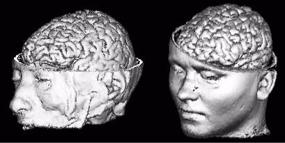
15 15 viewpoint by using the substances depth and intensity buffers. For any clipping polygon in 3D object space, we can use Eq. [4] to transform the vertices into view space. Once in view space, the BSR algorithm uses orthographic projection to project the vertices onto the view screen and a scan-conversion algorithm (14) to determine the interior pixels of the clipping polygon. While scan-conversion proceeds, other numbers associated with the vertices can be interpolated. Thus, we can quickly interpolate original voxel positions in object space corresponding to the clipping polygon. For each interior pixel of the clipping polygon we use two clipping buffers (in view space) to store: (1) the depth of the clip plane in view space and (2) the voxel in object space corresponding to the pixel. For each pixel in the view screen, the substances are traversed and composited in FTB order. When the clip plane is reached, two types of information may be depicted: (1) the image intensity I() p of an associated voxel is used if the the voxel corresponds to a substance or (2) a user-chosen clip plane intensity is composited. The former allows painting of image intensities onto clipped surfaces while the latter permits the highlighting of the clipping polygon. Results and Discussion The BSR algorithm has been extensively tested with over three dozen segmented images based on MR as well as CT and user-constructed volumes. Execution times vary with the size of the dataset and the user-specified parameters. In this section, we give example timings using two test images (Figure 7). The first test dataset uses a 3D MP-RAGE MR image of a cadaver head with five labelled objects: gray matter, white matter, ventricular system, ocular chambers (only for test purposes), and head which includes all foreground voxels not associated with the previous objects. The second test dataset uses a 3D MP-RAGE MR image of a volunteer with six labelled objects: right and left cerebrum, right and left cerebellum, brain stem, and head. The composition of each dataset is shown in Table 2. Sample times for each stage in the rendering process are shown in

16 16 Table 3 using a HP 9000/735 workstation. While full traversal of the pipeline for a new view takes slightly more than three seconds, clipping plane movement occurs at a substantially higher rate depending on the size of the clip polygon on the view screen. Small polygons showing an image intensity window can be moved at over 15 frames per second. The BSR approach assumes prior segmentation and the availability of labels λ( p). Multiple substances are handled using intermediate image buffers and a well-structured pipeline. Provisions are made for showing the I() p associated with clipped surfaces as described above; therefore, the BSR algorithm allows some degree of volume rendering. Given the large size of 3D medical images, BSR fortunately does not require interpolation to isotropic voxel size; a splatting stage is used after voxel projection. The renderer has been designed with particular attention to the needs of the neurosurgeon. Different medical specialties have different requirements, and with neurosurgery, interactive exploration of objects 3D relationships is critical. BSR, through the use of multiple substance buffers, is optimized for the rapid display of 3D object surfaces together with interior image intensities. This caching of intermediate results with real-time compositing can be used with any front-end rendering method such as ray casting (15) or shell rendering (16). Acknowledgements The authors would like to thank Jim Bertolina for his help in providing the images for this study. The work has been partially supported by the Medical Scientist Training Program, University of Virginia.

17 17 References 1. Goble JC, Snell JW, Katz WT. Semiautomatic Model-Based Segmentation of the Brain from Magnetic Resonance Images. Proceedings of AAAI Spring Symposium on Applications of Computer Vision in Medical Image Processing, March 1994, pp Fuchs H, Kedem ZM, Uselton SP. Optimal Surface Reconstruction from Planar Contours. Comm. ACM 20, (1977). 3 Herman GT. The Tracking of Boundaries in Multidimensional Medical Images. Comput. Med. Imaging Graph. 15, (1991). 4 Kaufman A (Ed.). Volume Visualization. Los Alamitos: IEEE Computer Society Press, Tiede U, Höhne KH, Bomans M, Pommert A, Riemer M, Wiebecke G. Investigation of Medical 3D-Rendering Algorithms. IEEE Comput. Graph. Appl. 10(2), (1990). 6 Foley JD, van Dam A, Feiner SK, Hughes JF. Computer Graphics: Principles and Practice. Addison-Wesley, Reading, Rogers DF, Adams JA. Mathematical Elements for Computer Graphics. McGraw-Hill, New York, Watt A, Watt M. Advanced Animation and Rendering Techniques. ACM Press, New York, Frieder G, Gordon D, Reynolds RA. Back-to-Front Display of Voxel-Based Objects. IEEE Comput. Graph. Appl. 5(1), (1985). 10 Reynolds R, Gordon D, Chen L. A Dynamic Screen Technique for Shaded Graphics Display of Slice-Represented Objects. CVGIP. 38, (1987). 11 Chen LS, Herman GT, Meyer CM, Reynolds RA, Udupa JK. 3D83 - An Easy-to-Use Software Package for Three-Dimensional Display from Computed Tomograms. Proc. of IEEE Comp Soc Int l Symp. Med Img & Icons 1984; pp Westover L. Footprint Evaluation for Volume Rendering. Comp Graph. 24, (1990). 13 Rogers DF. Procedural Elements for Computer Graphics. McGraw-Hill, New York, Heckbert PS. Generic Convex Polygon Scan Conversion and Clipping. In Graphics Gems (A.S. Glassner, Ed.), pp Academic Press, Boston, Levoy M. Efficient Ray Tracing of Volume Data. ACM Trans. Graph. 9, (1990). 16 Udupa JK, Odhner D. Shell Rendering. IEEE Comput. Graph. Appl. 13(6), (1993).

18 18 Table 1: Properties of a substance used in rendering. Parameter Range of values Meaning Color [0,0,0] to [1,1,1] 3D vector with red, blue, and green intensity components. Surface character Rough, normal, or smooth Selects different methods of computing a gradient vector. Visibility On or off Flag for inclusion of substance. Permeability On or off Flag for permeability of substance to the clipping plane. Opaqueness, α 0.0 to = transparent substance 1.0 = fully opaque substance Ambient lighting, I a 0.0 to 1.0 Constant light intensity added to the light reflected off a substance surface. Diffuse Reflectivity, k d 0.0 to 1.0 Degree that the substance is a perfect diffuser of incident light. Specular Reflectivity, k s 0.0 to 1.0 Degree that the substance is mirror-like. Center 0.0 to 1.0 The image intensity mapped to the display device s middle intensity. Window 0.0 to 1.0 The width of image intensities mapped to the display device s intensity gamut. Table 2: Composition of test datasets. Voxels Image Object Surface Total 1. Cadaver Gray Matter 423, ,799 White Matter 312, ,032 Ventricular System 9,368 12,000 Ocular Chambers 2,944 3,139 Head 518, ,447 Total 1,267,168 1,635, Normal Subject Right Cerebrum 78, ,603 Left Cerebrum 81, ,395 Right Cerebellum 12,971 34,736 Left Cerebellum 14,594 35,219 Brain Stem 4,925 11,012 Head 536, ,094 Total 729,096 1,600,059

19 19 Table 3: Execution Times for the Rendering Pipeline a Rendering Stage Time (seconds) for Image 1 (Figure 7a) Surface determination Voxel projections Splatting of footprint Shading & compositing (new view) Total for a new view Total for 1 y-axis rotation of old view Clip plane manipulation b 0.06 to to 0.3 Compositing of old view c 0.44 to to 0.94 Time (seconds) for Image 2 (Figure 7b) a. Timings are based on a HP 9000/735 workstation with 160 MB primary memory. b. Execution time is dependent on the size of the clipping polygon projected onto the view screen. Time given is for one translation or rotation of the clipping polygon. c. Compositing is the only stage executed when altering most substance properties. Execution time varies with the number of visible substances.

20 22

21 23 Computed once for each 3D image Ip ( ) λ( p) Determine surface voxels, normals, and neighbors. T V V S Computed once for each viewpoint Calculate voxel footprint in display space Project point onto the display plane Splat projected voxel using its footprint Compute shading using stored image gradients Composite substance buffers Ip () Computed interactively Rendered Image

22 24

23 25

24 26 (a) Head (b) Right cerebrum (c) Left cerebrum (d) Right cerebellum (e) Left cerebellum (f) Brain stem (g) Final composited view

25 27

26 28