Kingsoft Spreadsheet 2012

Transcription

1 Kingsoft Spreadsheet 2012 Kingsoft Spreadsheet is a flexible and efficient commercial spreadsheet application. It is widely used by professionals in many fields such as: Business, Finance, Economics and so on. It features calculation, graphing tools, and many other tools for complex data analysis. Kingsoft Spreadsheet supports more than 100 commonly used formulas and has a battery of supplied functions (conditonal expressions, sorting, filtering and consolidating for example) to make it much more convenient to analyze data. Kingsoft Spreadsheet has a variety of spreadsheet templates that make creating all kinds of spreadsheets quick and easy. Kingsoft Spreadsheet is completely compatible with all Microsoft Excel files and is also capable of outputting other file formats such as.txt,.csv,.dbf and more.

2 Catalog Kingsoft Spreadsheet Basic Operation Kingsoft Spreadsheet Brief Introduction Kingsoft Spreadsheet Interface Basic Operation Operate Cells Edit Spreadsheet Multiple summary results in the status bar Smart Contraction AutoComplete Function Home tab Clipboard Paste Cut Copy Format Painter Font Font Format Border Patterns Alignment Text alignment Wrap Text Join Cells Adjust Indent Number Quick Set Format Cell Format Style... 23

3 1.5.1 Conditional Formatting Style Cells Rows or Columns Operation Cell Editing Worksheet Operation Convert Text to Numbers and Convert to Hyperlink Editing Fill Clear Sort and Filter Find and Replace Text Insert Tab Tables PivotTable Chart Options Chart Chart Type Chart Structure Create Chart Custom Illustrations Insert Pictures Hyperlink Create hyperlink in WPS spreadsheet Group Create and Cancel Hyperlinks Text Text Box Header & Footer Insert Object... 64

4 3 Layout Tab Page Setup Margins Paper Orientation Paper Size Print Area Breaks Print Title Page Zoom Arrange Object Hierarchy Align Group Rotate Shift Formulas Tab Formulas Grammar Create Fomulas Input Formulas Copy a Formula Function Library Insert Function Use Functions in the Table Function Category AutoSum Define Names Define Cell Name Define Cell Range Name Define Formula Name Calculation... 96

5 4.4.1 Recalculate Active Book Manual Recalculation Iteration Data Tab Get External Data Import Data Edit OLE DB Query External Data Range Properties Refresh Data and Refresh All Data Tools Text to Columns Duplicates Validation Consolidate Outline Review Comments Create Comment Edit Comment Delete Comment Changes Lock Cell Protect sheet Protect Workbook Share Workbook Protect Shared Workbook Allow Users to Edit Ranges Track Changes View Workbook View

6 7.1.1 Normal Print Preview Page Break Reading Layout Freeze

7 Kingsoft Spreadsheet Basic Operation 1.1 Kingsoft Spreadsheet Brief Introduction Kingsoft Spreadsheet is an independent and powerful spreadsheet application that is a component of Kingsoft Office Kingsoft Spreadsheet does not only fulfill your daily needs of analyzing data, but can also help you to perform more professional data processing tasks. 1.2 Kingsoft Spreadsheet Interface If you have worked with any Windows programs or Microsoft Excel before, you are already familiar with the Kingsoft Spreadsheet user interface. It has all of the standard window components, such as the title bar, menu bar, status bar and so on. Title Bar: The title bar displays the name of the workbook. When you create new workbooks, the system will automatically name your workbooks as Book1, Book2 and so on. Menu Bar: The menu bar contains different commands that you can use to edit the worksheet. Name Box: The name box displays the selected cell address. If you select more than one cell, it will display the selected range address. Edit Bar: You can use the edit bar to edit the data in the cell. The edit bar will display the content you are editing in the cell. Rows: The rows are labeled with the numbers 1 to Document tab: You can easily switch between multiple documents by clicking the document tab. Columns: The columns are labeled with letters in the following pattern: A, B, C,... Z, AA, AB, AC,... AZ, BA, BB, BC,... BZ, CA,... IA, IB,... IV, which is the last possible column. Active Cell: The active cell has a dark border around it and the row and column headers are either raised or like buttons. This is the cell that receives your keystrokes and commands.

8 1.3 Basic Operation Operate Cells A cell is the basic unit for storing data in the spreadsheet. You can select, copy, cut, paste, edit, clear, move or join cells Edit Spreadsheet Input Text or Numbers There are two types of data in Kingsoft Spreadsheet: Text type data (characters, or the combination of characters and numbers) and numeric type data. All numeric values can be used to make calculations. In Kingsoft Spreadsheet, the data in text format will be aligned to the left, and the data in number format will be aligned to the right by default Input Text In Kingsoft Spreadsheet, text refers to the characters or the combination of numbers and characters. To input data in text format, enter ' ' ' before you enter the text data Input Numbers Numbers are composed of the digits 0-9 and some special characters such as: +, -, $, %, etc. There are several tips to consider when inputting numbers: When you enter a positive number, you do not have to add a '+' before the number. Even if you add it, it will automatically be omitted. When you enclose a number in "()", or parentheses, it means you have input a negative number. For example: (123) refers to If you want to enter a fraction, you should add a '0' before it, otherwise the system will display it as date. For example, if you want to input 1/2, you should input 0 1/2. There should be a blank space between 0 and 1/2. Otherwise it displays 2-Jan. When the input number is longer than the cell width or more than 11 digits, it automatically displays in scientific notation.

9 Input Date and Time When you input data, you can use '/' or '-' to separate the year, month and day. For example, '11/4/19' or ' '. To input time, you can use ':' to separate hours, minutes and seconds. For example, '9:30' and '10:30 AM". There are several tips you should pay attention to: In Kingsoft Spreadsheet, the date and time are treated as numbers, which means you can perform calculations with them. If you want to enter a 12-hour time, you should add 'AM' or 'PM' after the time. Otherwise it will be treated as a 24-hour time. If you want to enter the time and date in to the same cell, you should use a blank space to separate them. For example, ' :30" Enter the same data in to a discrete area To enter the same data in to a discrete area, follow the steps below: (1) Hold down CTRL and click the cells you wish to enter the same data in to. (2) Enter the data in to the active cells. (3) Press Ctrl+Enter Multiple summary results in the status bar In Kingsoft Spreadsheet, multiple summary results appear in the status bar if you select several numbers at a time. Some of these summary results include: Sum, Count, Min and Max.

10 Figure multiple summary results The four summary results mentioned above are defaults in Kingsoft Spreadsheet. To adjust any of them, you can right-click the status bar. The option list appears and you can add or delete the summary results according to your needs Smart Contraction Sometimes we have to enter too much information in a cell, and that makes it inconvenient to check information in other cells. Kingsoft Spreadsheet provides a smart contraction feature to make the aforementioned situation much easier to deal with.

11 Figure Smart Contraction AutoComplete Function The AutoComplete Function makes it easier to enter the same or similar data into different cells. This can improve the speed and efficiency of data entry. Operation steps are shown as follows: (1) Find the Application menu and click Options in the lower right corner. (2) Select the Edit tab from the Options dialog box and click the Enable AutoComplete for cell values check box. This process is shown as follows:

12 Figure Select Enable AutoComplete for cell values check box (3) When you enter the first character of similar content, the system will automatically provide a drop-down list for you to choose from. 1 Home tab 1.1 Clipboard After selecting the text or object, you can move, copy, delete and carry out various other commands on the selected content. You can complete all of these operations through the control command, the shortcut keys or the mouse Paste Paste refers to moving the contents from the system clipboard to the file at the designated insertion point. The paste operation can only be performed if the clipboard is not empty. To paste contents, follow these steps: (1) Look under the Home tab for the Clipboard group and click the Paste drop-down

13 arrow. User Manual Figure 1.1 1Paste (2) Kingsoft Spreadsheet provides five different methods of pasting content. Formulas:Paste the formulas contained in a data set rather than the data itself. No Borders:Paste the cell contents only, not with the cell borders. Values:Copy the selected cells containing formats and formulas and select the values button in the paste menu. By doing this, you can paste the values in the cells without altering the formats and formulas. Transpose:To rearrange row data to be displayed in columns, you should choose the Transpose option in the paste menu. Copy the selected row data and choose Transpose in the desired position to complete the action. Paste special includes the options mentioned above. However, you can also choose paste special from the paste menu directly, which allows for even more options to become available. Just right-click and choose paste special in the shortcut menu and the following paste special dialog box will pop up:

14 Figure ste Special Dialog box (3) You can press Ctrl+V to paste. This paste method pastes all copied content to the designated area. (4) Right-click on the document to open up the shortcut menu, you can then select paste Cut Cut refers to removing the currently selected contents within the file, and moving them to the system clipboard. From here, you can paste these contents to other places. To use the cut function, follow these steps: (1) Look under the Home tab for the Clipboard group and click Cut. (2) Use the keyboard shortcut Ctrl+X. (3) Right-click the selection and select Cut from the shortcut menu Copy Copy refers to duplicating the currently selected contents to the system clipboard, so that you can paste these contents to other places. However, the selected contents are still retained in the file. Using any of the following methods performs the copy function: (1) Click the Copy Button in the Clipboard group under the Home tab. (2) Use the keyboard shortcut Ctrl+C to copy the selection. (3) Select Copy in the shortcut menu by right-clicking the selection.

15 1.1.4 Format Painter Format Painter is a commonly used tool to replicate formats. It can replicate the format of selected objects, text or cells, and apply it to the corresponding content you select. (1) Put the cursor on the cells or objects that will have their format replicated. (2) Click the Format Painter button in the Clipboard group under the Home tab. (3) The mouse pointer will become the shape of the Format Painter. (4) Move the mouse to the object or cells to be formatted; select them and the operation can then be completed. Tips:If you want to use format painter continuously, you can double-click the Format Painter button so it becomes highlighted as shown. 1.2 Font The content of different cells can be set in different font formats, borders, fill colors, etc., according to the users needs. All of these things make it easy to recognize the content you want to highlight or emphasize Font Format The font format setting refers to set the font, size, style, color and so on Font Kingsoft Spreadsheet provides a variety of fonts to choose from. There is an appropriate font for different tastes, situations and requirements. To set the font, do the following: (1) Select the cell or text, which you want to set the font for. (2) Click the Font drop-down list in the Font group under the Home tab and select an appropriate font. The list is shown in the following figure:

16 Figure Set Font Font Size steps: Different font sizes can be used within a single document. To set the font size, take the following (1) Select the cell or text. (2) Click the Size drop-down list in the Font group under the Home tab and select the appropriate font size. You can also input numbers between 1 and 1638 in the drop-down list box and press Enter. It is also possible to quickly Increase and Decrease the font size. These buttons can be found under the Home tab and in the Font group Font Style Font style represents the format of the characters within the text. There are several commonly used control buttons in the Font group. These buttons are used to set the font style of the selected text. The functions of these buttons are as follows: Bold:Sets the selected text in bold or cancels the setting if the text is already in bold. Italic:Sets the selected text in italic or cancels the setting if the text is already in italic. Underline:Sets an underline for the selected text or cancels the setting if the text is already

17 underlined. User Manual Font color:set an appropriate color for the selected text. Click the button on and open the drop-down list to make a selection Border The color of the grid lines on the worksheet is gray by default. Grid lines are not displayed when you print, but if you need to print the grid lines, you should set borders for them. Take the following steps to set borders: (1) Select cells you want to set borders for. (2) Click the border drop-down list in the Font group of the Home tab and select different borders from the list. This list is shown in the following figure: Figure Border drop-down list Draw Border: Select Draw Border from the drop-down list and a pen tool will show up. This tool will allow you to draw an outside border for the selected cell ranges. Draw Border Grid: Select Draw Border Gird from the drop-down list and a pen tool

18 will show up which will allow you to draw a border grid for the selected cell ranges. Erase Border: Select Erase Border and an eraser tool will show up. You can then erase the border of selected cell ranges. Line Color: Set different colors for the border line. Line Style: Set different styles for the border line. Other Borders: Select Other Borders and the Cell Format dialog box will appear. Choose the Border tab. You can set the border line and choose the border style manually according to your requirement. An alternative to the method mentioned above is to set cell borders through the Format Cells dialog box: (1) Select cell ranges. Click the border drop-down list in the Font group under the Home tab. Choose the Border tab in the Format Cells dialogue box. (2) You can set the print display of the outside border and inside border from the Preset group. (3) Select the style of border lines from the Style drop-down list. (4) Select the color of border lines from the Color drop-down list. (5) You can complete all these setting by pressing the OK button. Figure Set the border in the Format Cells dialog box

19 1.2.3 Patterns User Manual You can set shading for selected cells. Click the drop-down arrow near the Patterns button and select the fill color you desire from the Patterns list box. You can also complete the cell shading setting mentioned above by following these steps: (1) Select the cell or cell range that you want to apply shading to. On the Home tab, in the Font group, click the Old Tools button on the lower right corner. The Format Cells dialog box will appear as shown in the following: Figure Patterns Tab (2) Choose the Patterns tab in the Format Cells dialog box and several options will become available. Background Color controls cell shading color; Pattern Style controls the style of patterns and Pattern Color controls the color of patterns. (3) Press the OK button. You can select the cell or cell range and right-click, then open the short-cut menu and select Cells and the Format Cells dialog box will pop up. 1.3 Alignment Text alignment Select a cell or a cell range, go to the Home tab, find the Alignment group and click Alignment.

20 Kingsoft Spreadsheet provides three kinds of alignment: Align Left, Center and Align Right. You can also set the border of cells by using the Format Cells dialog box. Steps are shown as follows: (1) Select the cells you want to align. (2) On the Home tab, in the Alignment group, click Old Tools in the lower right corner. (3) In the Format Cells dialog box, under Alignment, in the Text alignment group, select an appropriate Horizontal and Vertical alignment. (4) Press OK Wrap Text Figure Set Alignment in the Format Cells dialog box If you need to input more than one line of data into a cell, take the following steps: (1) Select the cell with data you want to wrap. (2) On the Home tab, in the Alignment group, click Wrap Text, and set the content. Aside from the way mentioned above, you can wrap data through the Format Cells dialog box. Operation are shown as follows: (1) Select the cell with data to be wrapped. (2) On the Home tab, in the Alignment group, click Old Tools in the lower right corner. (3) The Format Cells dialog box pops up. Under Alignment, click the check box labeled as: Wrap text in the Text control group.

21 Figure Wrap Text (4) Click OK. The keyboard shortcut, Alt+Enter also performs this function Join Cells There are four options in the Join and Center drop-down list: Join and Center, Merge Columns, Join Cells and Columns Center. On the Home tab, in the Alignment group, select options in the Join and Center drop-down list. These options make the process of merging cells much quicker and easier. Figure displays this. Figure Join and Center Join and Center:Selected cells will be joined and the content they include will be aligned to the center. Merge Columns:Selected columns and rows will be merged, but the number of rows will

22 not change in this case. Join Cells:Joins the selected cells. Columns Center:The content in every cell will be aligned to the center, but cells will not be joined. The alignment standard is based on the longest cell selected. You can join or disjoin cells in the following way: select the cell or cells; click Join and Center under the Home tab, in the Alignment group. You can also join or disjoin cells in the Format Cells dialog box. This is explained in the following steps: (1) Select the cells that need to be joined or disjoined. (2) On the Home tab, in the Alignment group, click Old Tools in the lower right corner. (3) Choose the Alignment tab in the Format Cells dialog box and check or uncheck Join cells in the Text control group. Figure Join cells in the Format Cells dialog box (5) Press Ok Adjust Indent To change the indent of the cell content, you can use the Decrease Indent and Increase Indent

23 functions in Kingsoft Spreadsheet. (Indent refers to the margins between the border and text) Look under the Home tab for the Alignment group and select Decrease Indent. This reduces the distance or margin between the cell border and the content. Look under the Home tab for the Alignment group and select Increase Indent. This increases the distance between the cell border and the continent. 1.4 Number Quick Set Format You can easily set the format of selected cells in the Number group. There are several control buttons in the Number group, such as: Currency, Percent Style, Comma Style, Increase Decimal and Decrease Decimal. Currency:Add a currency format for the selected cell(s). Percent Style:Display the values in the selected cell(s) as percentages. Comma Style:Add commas to the data in the selected cell(s). Increase Decimal:Display the data in higher accuracy by increasing the decimal digits. Decrease Decimal:Display the data in lower accuracy by decreasing the decimal digits Cell Format There are 12 categories for cell format properties. These categories are: General, Number, Currency, Accounting, Date, Time, Percentage, Fraction, Scientific, Text, Special and Custom. There are several ways to bring up the Format Cells dialog box in order to set the format properties of each cell. Look under the Home tab for the Number group and select Cells. The Format Cells dialog box will appear and the Number tab will become available. Look in the Home tab for the Number group and click Old Tools in the lower right corner. The Format Cells dialog box pops up and the Number tab will be available. Press Ctrl+l to make the Format Cells dialog box appear and select the Number tab. You can choose a format type from the Category list found in the Number tab. When you choose a

24 different format type, there will be different information references displayed on the right side of the window. You can adjust according to the references in order to achieve a custom effect. General The General format is the default number format when you type a number into a cell. The general format does not include any special format for numerical values. Number Select Number from the Category list and a sample box on the right side of the window will appear. This sample box previews the changes in decimal, comma, and negative value usage made to the number format. This is displayed in Figure Figure Number format and options After selecting the Number Category, you can adjust the following settings in the dialog box: Decimals can be added to the number format as well as 1000 separators. You can set the negative number formats in the Negative numbers list box. Currency Select Currency from the Category list and a sample box on the right side of the window will appear. This sample box previews the changes in decimal, currency symbol and negative value usage. This is displayed in Figure

25 Figure Currency format and options After choosing Currency, you can set the basic display style for currency in the dialog box. These display settings allow you to customize Decimal digits, the Currency Symbol and the display format of Negative numbers. Accounting Choose Accounting in the Category list box. The sample box on the right displays the format setting options. You can define the basic accounting display format by customizing the Decimal digits, Symbol, etc. Figure displays the Accounting format and options. Figure Accounting format and options

26 Date User Manual Select Date in the Category list and you will be able to preview the type of date in the sample box on the right. This is displayed in Figure Figure Date format and options Time Select Time in the Category list. The sample box on the right displays the format setting options. This is shown in Figure Figure Time format and options

27 Percentage User Manual Select Percentage in the Category list. The sample box on the right displays the format setting options. This is shown in Figure Figure Percentage Fraction Select Fraction in the Category list. The sample box on the right displays the format setting options. This is shown in Figure Figure Fraction format and options

28 Scientific User Manual Select Scientific in the Category list. The sample box on the right displays the format setting options. This is shown in Figure Figure Scientific format and options Text Select Text in the Category list. You can convert decimal numbers into text. Special Select Special in the Category list. There are three types of special formats, such as: Zip code, Zip Code + 4 and Social Security Number. Figure Special Format

29 Custom User Manual list box. Select Custom in the Category list. You can set various kinds of customized data formats in the Type 1.5 Style Conditional Formatting You can set conditions for cells. When cells meet these conditions, the program will automatically apply some type of formatting to them. You can set three conditions at a time and can choose to use formulas or cell values as the conditions. For example: Change the color of the cell to yellow when the date in the cell matches the current date. This function can be used to remember the birthday of friends or employees. To set a condition, do the following: (1) Select the data. (2) On the Home tab, in the Style group, click Conditional Formatting. The Conditional Formatting dialog box pops up. (3) Select Cell Value Is in the Condition drop-down list. Select equal to. Input '=today()' in the edit box as shown in the following figure: Figure Conditional Formatting dialog box (4) Click Format and the Format Cells dialog box pops up. You can set the display format for the cells. (5) Press OK.

30 1.5.2 Style User Manual In Kingsoft Spreadsheet, you can use the directly built-in styles. To use these styles, follow these steps: (1) Select cells you want to apply a style to. (2) On the Home tab, in the Style group, click Style. The Style dialog box will pop up: Figure Style dialog box (3) There are six styles in the Style name drop-down list: Comma, Comma[0], Currency, Currency[0], Normal, Percent. (4) The Style includes group lists all the styles included. If you need to modify any specified format, click Modify and the Format Cells dialog pops up. You can then reset the format. (5) Press OK. 1.6 Cells Rows or Columns Operation You can change the structure of the worksheet by performing operations on it. The main operations include: Select, Display, Hide, Insert, Delete, Move columns or rows Select Rows or Columns If you want to delete or move rows or columns, you should select them first. Click the row number or column label to select one row or one column. You can select one row or column first, then press SHIFT

31 and click another row number or column label at the same time. By doing that, you can select two rows (or columns) or more which are adjacent. An alternative is to press CTRL and click different row numbers or column labels at the same time. By doing that, you can select more than one row (or column) which are non-adjacent Hide or Unhide Columns or Rows If you don't want other people to see some particular content in your worksheet, you can hide the rows or columns that contain the content. The steps to hide rows or columns are as follows: (1) Select rows or columns. (2) On the Home tab, in the Cells group, click Hide/Unhide in the Format drop-down list. Point to Hide Rows or Hide Columns. Shown as follows: Figure Hide and Unhide list If you want to unhide rows or columns, you can follow the same steps mentioned above. Choose Unhide Rows or Unhide Columns. Select rows or columns. Right-click. Select Hide or Unhide in the shortcut menu. Then you can perform the hide or unhide function Move Rows or Columns If you want to adjust the display order of rows or columns, you can move their positions. To do so, follow these steps: (1) Select the rows or columns you want to move. (2) Move the mouse to the border of the selected rows or columns. When the shape of the mouse changes from an arrow to a cross, you can drag the mouse to the specified place. (3) Release the mouse and then you can move the position of the rows or columns.

32 Insert Rows or Columns On the Home tab, in the Cells group, there are four options in the Insert drop-down list: Insert Cells, Insert Rows, Insert Columns and Insert Sheet. Insert Rows will be used as an example to introduce the necessary steps to insert these options. (1) Select the location to insert rows. (2) Choose Insert Rows from the Insert drop-down list in the Cells group. You can then insert a row in the worksheet. This is shown in the following picture: 1.Select the position you want to insert the row 2,In the Cells group, click Insert,and select Insert Rows. Rows

33 The effect after inserting Figure Insert Rows Insert columns works the same way as insert rows Delete Rows or Columns You can delete any unwanted rows or columns in the following two ways: Select the unwanted rows or columns. On the Home tab, in the Cells group, select Delete Rows or Delete Columns from the Delete drop-down list. Then you can delete selected rows or columns. This is shown in Figure Figure Delete list Select the unwanted rows or columns. Right-click. Choose Delete in the shortcut menu Row Height and Column Width Setting You can adjust the height of the rows and width of the columns if you feel they are not suitable at the default size. Follow these steps to set the row height and column width. (1) Select the rows or columns. (2) On the Home tab, in the Cells group, select Height or Width from the Format drop-down list. This is displayed in Figure

34 Figure Set the Row Height and Column Width (3) You can set row height or column width in the Row Height or Column Width dialog boxes. (4) Press OK. You can also accomplish this by doing the following: Select the rows or columns. Right-click. Choose Height or Width in the shortcut menu. 1.7 Cell Editing You can insert, delete, copy and modify worksheets Worksheet Operation There can be multiple worksheets in the workbook and new worksheets can be inserted at any time. You can also copy, paste, move, rename or delete worksheets Select the Worksheet If you want to move, copy, cut or delete the worksheets, you have to select them first. If you want to select a single worksheet, click the worksheet label.

35 Figure Select a single Worksheet When you hold down SHIFT and try to select worksheets, you can select multiple worksheets that are adjacent to one another. However, when you hold down CTRL and try to select worksheets, you can select multiple worksheets that are non-adjacent to each other. Select all the Worksheets Figure Select all the Worksheets Move and Copy Worksheet There are two ways to move and copy worksheets: Move/Copy Sheet in the Format drop-down list or you can use your mouse. Move or copy worksheets by using the Edit menu. (1) Open and select a worksheet. (2) On the Home tab, in the Cells group, select Move/Copy Sheet in the Format drop-down list. Then the Move/Copy dialog box as shown in Figure appears.

36 Figure Move/Copy Sheet (3) In the To book drop-down box, select the workbook you want to put your worksheet in. If you want to move or copy the selected worksheet into the new workbook, select New book. (4) Select the worksheet that you want to insert or copy in the Before Sheet list box. (5) If you want to copy rather than move the worksheet, click the Create a copy check box. (6) Click OK to finish all of the copying or moving operations. Move or copy worksheets by using the mouse. This method is suitable for copying or moving worksheets that are in the same workbook. Steps to doing so are as follows: (1) Select the worksheets that you want to move. To move the sheets in the current workbook, you can drag the selected sheets along the row of sheet tabs. When you drag the selected sheets there will be a little dark triangle on the top left of the first tab. The little dark triangle indicates the location of the worksheet. (2) Select the worksheets that you want to copy. To copy the sheets, hold down CTRL, and then drag the sheets to the position you want them be. (3) When the little dark triangle moves to the correct position, you can release the mouse button before you release the CTRL key. You can also release the mouse button and CTRL key at the same time. (4) Figures and depict the process of moving a worksheet.

37 Figure Before moving Figure After Moving Figure indicates how a worksheet is copied. Figure Copy the worksheet Insert and Delete Worksheet When using Kingsoft Spreadsheet, you will probably have to insert new worksheets or delete spare worksheets. (1) Insert Worksheet If you want to insert one or more worksheets, take the following steps: (1) Select the current worksheet.

38 (2) There are two ways to insert a worksheet: I: On the Home tab, in the Cells group, select Insert Sheet from the Insert drop-down list. II: Right-click the worksheet label, and select Insert. (3) The Insert Sheet dialog box appears. Enter the number of worksheets you want to create. Under the Insert group, select the location you want to insert the new worksheet, there are two options: After current sheet and Before current sheet. Figure Insert Sheet dialog box (4) Press OK. (2) Delete Worksheet If some worksheets are unnecessary, you can delete them. To do so, follow these steps: (1) Select the worksheet you want to delete. (2) There are two ways to delete worksheet: I: On the Home tab, in the Cells group, select Delete Sheet from the Delete drop-down list. II: Select the worksheet label, right-click, and select Delete Worksheet from the shortcut menu. If there is data in the current worksheet, the following dialog box will be promoted. Figure Delete data in sheet (3) If you've made up your mind to delete the worksheet, you can press OK.

39 Rename Worksheet By default, Kingsoft Spreadsheet names worksheets after the model of 'Sheet + serial number'. In most cases, you would want to rename the worksheet. There are many ways to rename worksheets. The following are methods to rename worksheets. Double-click the worksheet label; enter the new name when the label is in the selected status. Press Enter or click any place except the worksheet label to finish the renaming process. Right-click the worksheet label that you want to rename. Select Rename in the short-cut menu and enter the new name. Press Enter or click any area except the worksheet label to finish renaming the worksheet. Select the worksheet label, go to the Home tab, in the Cells group and select Rename from the Format drop-down list Hide Worksheet There are two methods to hide a worksheet. They are the following: Select the worksheet. Go to the Home tab, in the Cells group, click HideUnhide from the Format drop-down list and select Hide Sheet. Select the worksheet. Right-click and select Hide from the short-cut menu Convert Text to Numbers and Convert to Hyperlink Kingsoft Spreadsheet supports the mutual conversion between text and numbers. You can also Convert Text to Number and Convert Text to Hyperlink. When there is large amounts of data in text format, and you want convert them to numeric format, you can do the following: On the Home tab, in the Cells group, select Convert Text to Data from the Format drop-down list. When a large number of hyperlinks are not active, you can activate them by group. Select the contents you want to change to hyperlinks. Choose Convert to Hyperlink in the Format drop-down list.

40 1.8 Editing User Manual Fill To avoid entering large amounts of repetitive data manually, you can use the Auto Fill feature to fill cells in a more efficient manner Auto Fill There are two types of data series commonly used to fill cells in Kingsoft Spreadsheet. The first type includes: years, months, weeks, quarters and other text-type sequences. For text-type sequences, you just need to enter values in the first cell, then drag the fill handle to accomplish the filling. Operation steps are: (1) Select the cell range. (2) Move the mouse to the lower right corner of the data field and the pointer changes to a cross. (3) Drag the cross down to the last cell in the cell range. Then release the mouse button. The Auto Fill result is shown as follows: Figure Auto Fill The second type includes: 1,2,3; 2,4,6 and other numeric sequences. For numeric sequences, you need to enter the first two numbers that display the change pattern, and then drag the fill handle to fill in the specified pattern.

41 For non-sequence text (such as 'Office') and numeric sequences that don't specify the change pattern (such as 200), drag the fill handle to duplicate data. On the Home tab, in the Editing group, click Fill, and then click Down, Right, Up, or Left. This is shown as follows: Figure Fill list The difference between filling with duplicated data and filling with sequence data is: if you want to fill the cells with duplicated data, you have to press CTRL and drag the fill handle at the same time. If you only drag the fill handle, the system will automatically fill the cells with sequence data Fill data in worksheets of the same workbook Operation steps are as follows: (1) Select the data you want to fill into other worksheets within the same workbook. Figure Select the data you want to fill (2) Press SHIFT and CTRL at the same time. Select the worksheet you want to fill with data. (3) On the Home tab, in the Editing group, select Fill Across in the Fill drop-down list.

42 There are three options in the Fill Across dialog box: All: The same contents and formats will be filled and nothing will be changed. Contents: Only fill with the same contents while the existing formats remain. Formats: Only fill with the same formats while the existing data remains. (4) Select All and press OK. You can see all the contents in the worksheet. Figure displays this. Figure Fill effect Fill data by using a custom fill series To make entering a particular sequence of data such as a department name or an employee name easier, you can create a custom fill series. A custom fill series can be based on a list of existing items on a worksheet, or you can type the list from scratch. Operation steps are as follows: (4) Click Options in the Application menu. (5) In the Options dialog box, select Custom Lists tab. Shown as follows:

43 Figure Custom Lists (6) Select New List in the Custom Lists list box. (7) You can type the new list in the List Entries box on the right. You have to interlace every item in the list. (8) Click Add, then the new list will appear in the Custom lists box on the left. (9) Press OK. When you create a custom list, you can only input an item from the list into a cell. You then drag the fill handle and the remaining items will show up Clear Kingsoft Spreadsheet provides four types of clear options. All:Select the cells that you want to clear. Choose All from the Clear drop-down list. You can then clear all the contents in the cells. Formats: Select the cells that have formatting you want to clear. Choose Formats in the Clear drop-down list. Then you can clear the format, but the content will remain. Contents: Select cells that have content to be cleared. Choose Contents in the Clear drop-down list. All the contents are cleared, but the formats will remain. Comments: Select cells that have comments to be cleared. Choose Comments in the Clear

44 drop-down list. When the little red triangle disappears, this means cell comments have already been cleared. In Kingsoft Spreadsheet, you can clear comments in a cell as well as all of the comments in the spreadsheet Sort and Filter Sort At times, it is better to have the worksheets in your workbook arranged in a specific order. Doing so makes it easier to navigate through your document. The sorting feature makes this possible and allows you to arrange the data in your rows and columns in descending and ascending order. The sorting operation steps are as follows: (1) Click any cell or cells in the worksheet you want to sort. (2) On the Home tab, in the Editing group, select Sort in the Sort and Filter drop-down list. The Sort dialog box will appear. Figure Sort dialog box (3) Select the corresponding keyword and field in the Sort drop-down list. (4) Press OK. The records in the worksheet will be sorted by the keyword you set. This is displayed in Figure

45 Figure Sort by Keywords Filter Filtering data is a quick and easy way to find and work with a subset of data in a range of cells or in a table. Filtered data displays only the rows that meet the criteria you specify and hides rows that you do not want to display Automatic Filter Automatic Filter makes it easy to find and process subsets of data in the spreadsheet. You can create criteria to filter data. Only rows that meet the criteria you specify will be displayed. Filtering doesn't rearrange rows; it is different from sorting. Filtering just hides the rows you don't want to display. Automatic filter includes: Simple Filter, Top 10 Automatic Filter and Custom Automatic Filter. In this chapter we'll introduce these three features. 1. Simple Filter Operation steps for simple filter are shown as follows: (1) Select the column(s) you want to filter. In the Editing group, select Automatic Filter in the Sort and Filter drop-down list. (2) Then a drop-down button shows in the first row of the column you select. (3) Click the drop-down list and you can set the filter. For example, click NB003 in the Name drop-down list. Shown as follows:

46 Figure Simple Filter (1) Then the column will be filtered by the keyword you selected. And all the rows that meet the criteria will be displayed. Shown as follows: Figure Filter effect 2. Top 10 Automatic Filter Operation steps for top 10 automatic filter are shown as follows: (1) Select data columns. In the Editing group, select Automatic Filter in the Sort and Filter drop-down list (2) In the Filter drop-down list, select Top 10. Shown as follows: (3) Figure Top 10 Automatic Filter (4) Then the Top 10 AutoFilter dialog box will pop up. Shown as follows:

47 Figure Top 10 AutoFilter (5) Enter the Show record, and click OK to finish. 3. Custom Automatic Filter If you want to create a criteria to filter by a data range, or filter by some comparison operators more complex than 'Equal to', you can customize the filtering. Operation steps are shown as follows: (1) Select data columns. In the Editing group, select Automatic Filter in the Sort and Filter drop-down list (2) In the Filter drop-down list, select Custom. Shown as follows: Figure Custom Automatic Filter (3) In the Custom Automatic Filter dialog box. Select the operation conditions and upper and lower limit values. Click OK. Figure Custom Automatic Filter

48 (4) The filter result is the wanted result. Shown as follows: Figure Filtering result If you want to restore the filtered data, you can select Show All in the Sort and Filter drop-down list. Then all the data will be displayed Advanced Filter The Advanced filter lets you use complex criteria to filter a range. And the filter result can be displayed in the original worksheet. The rows that don t meet the criteria will be hidden. The filter result can also be displayed in a new location. Operation steps are shown as follows: (1) In the Editing group, select Advanced Filter in the Sort and Filter drop-down list. The Advanced Filter dialog box pops up: Figure Advanced Filter dialog box Filter the list, in-place: hide data rows that don't fit the filter condition. And display the filter result in the original worksheet. Copy to another location: copy the data rows that fit the filter condition to another location. But the data rows that don't fit the filter condition will remain in the original worksheet and won't be hidden. By doing that, it's very convenient to compare the data. (2) Click Copy to another location, and check Unique records only. Shown as follows:

49 (3) User Manual Figure Before filtering Figure After filtering Reapply Figure Modify the data In the Editing group, select Reapply, in the Sort and Filter drop-down list. Shown as follows: Figure Filtering result

50 1.8.4 Find and Replace Text Find Text Operation steps are shown as follows: (1) On the Home tab, in the Editing group, select Find in the FindSelect drop-down list. The Find dialog box pops up. Figure Find Tab (2) Input the text you want to find, in the Find What box. Click Options, unfold the dialog box. Click Find Next, you can locate the cell. Click Find All, all the data which meet your requirement will be listed Replace Text Operation steps are shown as follows: (1) On the Home tab, in the Editing group, click Replace in the Find and Select drop-down list. Then the Replace dialog box will pop up. Click Replace tab. Figure Replace Tab (2) Enter contents you want to find, in the Find What input box; enter contents you want to replace with, in the Replace With input box.

51 (3) Click the Replace All button and replace all the content. Tips: You can enter nothing in the Replace With input box, and then you can delete all the contents which you are finding Go To You can quickly locate data in the cell by using the Go To feature which Kingsoft Spreadsheet provides. You can check options in the Go To dialog box, according to your need. On the Home tab, in the Editing group, select Go To in the Find and Replace drop-down list. Then the Go To dialog box will pop up. Shown as follows: Go To You can quickly locate data in the cell by using the Go To feature that Kingsoft Spreadsheet provides. You can check options in the Go To dialog box, according to your need. On the Home tab, in the Editing group, select Go To in the Find and Replace drop-down list. Then the Go To dialog box will pop up. Shown as follows: Figure Go to Tab

52 2 Insert Tab User Manual 2.1 Tables PivotTable PivotTables are dynamic tabulations that allow you to quickly combine and compare data to produce information tailored to suit your needs. In pivot tables, users can rotate rows and columns to view details from different perspectives. In brief, use pivot tables to simplify complicated data and discover an internal model that would otherwise be difficult to find in a disordered list. However, it is recommended to use pivot tables only when you have a long list of complicated data and want to analyze the related details. Otherwise it is not necessary to use this function. Operation Steps: (1) On the Insert Tab, in the Tables group, click PivotTable Figure Insert PivotTable (2) In the Create Pivot Table dialog box, choose the data range that you want to base your pivot table (If you already activated a cell in that source data range before performing the first step, Kingsoft Spreadsheets will automatically select that range for you) and the data range will be enclosed by dotted boarders. You can also modify a Pivot Table that already exists in the spreadsheet. Choose where you want the Pivot Table to be placed; there are two options: New Worksheet and Existing Worksheet.

53 Figure Create Pivot Table (3) After clicking OK in the Create Pivot Table dialog box, an empty pivot table appears in the specified sheet. If you want to put contents into it, please look to the Pivot Table task window on the right, which pops up automatically. Items in the Field List can be dragged to Page Area, Column Area, Row Area and Data Area in the Pivot Table Areas as you go. Moving to different areas means changing to a different viewing perspective, while moving out of any area deletes it from this area. Then you can analyze the detailed information contained in the data.

54 Figure Set for the Pivot Table (1) Right-click the fields in the task pane, and select Field Settings on the shortcut menu. You can then change the names or the ways of sorting the fields in the PivotTable Field. Figure Set the Pivot Table Field (1) You can drag fields outside the PivotTable Areas to remove. And you can also drag fields up

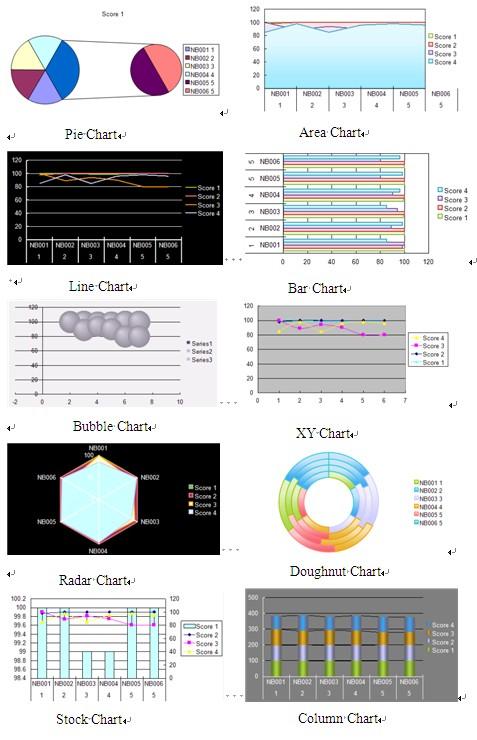
55 and down to adjust their position in the same data range. (2) On the PivotTable Tools Tab, in the Data group, click Delete PivotTable Figure Delete PivotTable 2.2 Chart Options In order to enhance the explanatory power of the data and make the data vivid for the reader, you can use the 'charts' to display data. Chart is the most intuitive way to analyze the data. Kingsoft Spreadsheet can automatically generate various kinds of charts according to the data in the cells, such as: Column chart, Bar chart, Line chart, Pie chart, Area chart and so on. All these types of charts can easily convert between one another. In the following section we'll introduce the structure of charts, how to create charts, how to set the advanced properties of tables and how to output charts Chart Charts provide a visual benefit by displaying comparisons, patterns, and trends in data, and help the user to analyze and compare data in an easy way. To see the comparison or trend, you do not need to analyze individually large quantities of data in the worksheet Chart Type Kingsoft Spreadsheets offers 11 types of charts, and you can choose the appropriate one to best convey what you want to express effectively. They include: Column chart, Bar chart, Line chart, Pie chart, XY(Scatter) chart, Area chart, Doughnut chart, Radar chart, Bubble chart, Stock chart, and Custom. And you can choose different styles and colors with each type of chart.

56

57 Figure Chart Type dialog box Chart Structure A chart is composed of the chart area and other elements in the area, such as the: chart title, legend, axes and so on. Some elements shown in the group such as the legend and data series for example, can be subdivided into separate elements. This is shown as follows: Elements of the chart: Data Source:Refers to the data range you select to create charts Data Series: Data series are automatically generated by the group of data that is going to be on the chart if you use the Chart Wizard. You can choose line data or column data to generate the series. Data Labels:To quickly identify a data series in a chart, you can add labels to the data point of the chart. By default, the data labels are linked to values on the worksheet; it can be values in the spreadsheet, or percentage and labels, etc. You can set the properties of data labels via the Data Labels tab of the Chart Settings dialog box. Axes:Axes are lines on the edge of the charts used to measure and compare data. Charts usually have two axes: a vertical value (y) axis, and a horizontal (x) axis. Chart Title:Chart titles are usually a short description of the chart, and it is usually found at the top center of the chart or aligns with the axes automatically. Legend:Displays the names of the data series and corresponding patterns and colors. Figure Structure of the chart

58 2.2.4 Create Chart User Manual The following steps show how to create a chart: (1) Select the cells that contain the data you want to plot in a chart. For example, select cell range A2: E6 in the worksheet below. Figure Select the data area (2) On the Insert Tab, in the Chart group, click Chart. The Chart Type dialog box will pop up. (3) Click the suitable chart type in Chart Types. In the following example we choose Clustered Column from the Column chart (4) Click the Next button, and the Source Data dialog box will pop up. There are two tabs in the dialog box: Data Range and Series. The Data Range tab is used to modify the data range of the chart. The Series tab is used to change the name, value and category (x) axis labels of the data range.

59 Figure Select the chart type Figure Set the data area (1) Click Next, then the Chart Settings dialog box pops up. There are 6 tabs: Titles, Axes, Gridlines, Legend, Data Labels and Data Table in the dialog box. Enter the corresponding titles in the boxes like Chart title, Category (X) axis, Value (Y) axis respectively. Click the

60 other tabs and choose the relative settings according to your needs.(for example, in the "Title" tab in the "Chart Title" text box, enter "2011 sales statistics" and in the "Value (Y) axis" text box, enter the units as "million" See examples of English screenshots) (2) Click Finish. You can then get the chart you want in the current worksheet. Shown as follows: Figure Chart Settings Figure Chart Custom Kingsoft Spreadsheet contains rich chart styles and a vibrant color scheme. Kingsoft also provides a custom chart option. When creating your own chart, you have the option to save them, so for future use

61 you can easily access your previously designed charts. When creating your own chart, you have the option to save them for future use. The following steps show how to create a customized chart: (1) Create a chart in the current worksheet. You can follow the steps we mentioned in chapter (2) On the Chart Tools tab, click Change Chart Type. Then the Chart Type dialog box pops up. Figure Chart Type dialog box (1) Click the button Add to custom type in the bottom to save your customized chart style. Shown as follows: (2) Add the name and description in the Add User-Defined Type dialog box. Shown as follows: Figure Add User-Defined Type

62 (3) Press Ok and finish the setting. After adding the customized chart type, you can see it in Custom within the Chart Type dialog box. Shown as follows: Figure Add to the Custom Type You can delete the customized chart type by selecting it in the Custom option within the Chart Type dialog box. Then click Delete to remove it from the Custom option. 2.3 Illustrations Insert Pictures If the table only contains raw data and text, there is a possibility for the data to appear monotonous and unimportant. Images can be used as an incredibly useful tool to display the data, allowing users to visually become aware of the contents of the data Insert from File If you have pictures on your computer which you feel would enhance the expression of the data, then you can insert these pictures into the worksheet. On the Insert Tab, in the Illustrations group, click Picture. Then the Insert Picture dialog box will pop up. Shown as follows:

63 Figure Insert the picture from File Find the path for the pictures in the "File Name" search box. Then click open; the pictures will be inserted in the current worksheet Insert from Clip Art If you can't find suitable pictures on your computer, you can select some from the built-in clip art. Kingsoft Spreadsheet provides abundant clip art resources for you to choose. On the Insert Tab, in the Illustrations group, click Clip Art. Then the Clip Art task window will appear on the right side of the spreadsheet. All you have to do is double-click the one you would like and the clip art will be added into the current workbook. Shown as follows: Figure Insert the Clip Art After inserting the pictures or clip art, the Picture Tools tab will appear after the Developer tab.

64 Insert from Shapes If pictures and clip art are not enough for you to express the meaning, you can use shapes. Kingsoft Spreadsheet provides all kinds of shapes. The shapes will enrich the data. On the Insert tab, in the Illustration group, click Shapes. Then the Shapes drop-down list will appear. Figure Shape list box After inserting the shape you picked, the Drawing Tools tab shows up. You can perform all kinds of operations to the shape such as; modify and many more. 2.4 Hyperlink Create hyperlink in WPS spreadsheet A link can be established with the cell. The cell can be associated other cells, files, web pages or even

65 a link between an account. Specific steps are as follows: (1) Select the cell you want to add a hyperlink to. (2) On the Insert tab, in the Links group, click Hyperlink. The Insert Hyperlink dialog box pops up: Figure Insert Hyperlink dialog box (3) In the Link to group, select the target file. (4) Press Ok. (5) Click on the cell you've already added a hyperlink to; you can link this to the target file immediately. Figure Cell with hyperlink To meet the different requirements of customers, Kingsoft Spreadsheet provides a hyperlink control tab. This means you can input information about the Internet or network path. You can decide whether the settings automatically set links to be changed into a hyperlink. The operation steps are shown as follows: (1) Open the Application menu on the top left corner. Click Options in the lower right corner.

66 (2) In the Options dialog box, select Edit tab. Shown as follows: Figure Edit Tab (3) In the Edit Settings group, set Replace Internet and network paths with hyperlinks as you type. If you click the check box, it will determine that the hyperlinks will be activated by default Group Create and Cancel Hyperlinks If on a document, Web or addresses are not hyperlinked, it is possible to group convert a hyperlink. You must use the Kingsoft volume conversion tool which will allow you to perform this function to facilitate your document or needs. Steps are as follows: (1) Only the URL or addresses can be a Hyperlink. So select the cell range which needs to be converted to a hyperlink. (2) On the Home tab, in the Cells group, click the Format drop-down list. Choose "Convert to Hyperlink" and finish setting.

67 Figure Then we can group convert Web URLs into hyperlinks If you want to remove the hyperlink, you can select the target cell range, right-click, then choose Remove Hyperlink in the short-cut menu. Shown as follows: Figure Remove Hyperlink

68 2.5 Text User Manual Text Box Kingsoft Spreadsheet provides two types of text: Horizontal Text Box and Vertical Text Box. On the Insert tab, in the Text group, you can select Horizontal Text Box or Vertical Text Box in the Text Box drop-down list. After selecting, you can drag your mouse to insert the text. In the text box, right-click, select the Format Text Box in the short-cut menu, then the Set Text box Format dialog box will pop up. You can set the format of current font. Shown as follows: Figure Set Text box Format Header & Footer On the Insert tab, in the Text group, click Header & Footer. The Page Setup dialog box will pop up. Choose the Header/Footer tab. You can set the customized header and footer.

69 Figure Header/Footer Tab You can set the format of the header or footer by selecting Custom Header or Custom Footer. And you can preview the resulting effect. Figure Header dialog box If you need to set the format of the text, put the cursor in the edit box, then click the Font button. If you need to insert Page, Pages, Date, Time, File, Tab, put the cursor in the edit box and press corresponding button. If you need to insert pictures, click the Insert Picture button. If you need to set the

70 format of pictures, put the cursor in the edit box, and click the Reset Picture button. After you have finished all the settings, press OK and exit. You can see the real effect, when back in the header/footer tab Insert Object The steps to insert an object is shown as follows: (1) On the Insert tab, in the Text group, click Object. The Insert Object dialog box pops up. Figure Insert Object dialog box There are two ways to insert objects: New:insert object directly. Select the object type in the Object Type drop-down list. Kingsoft Spreadsheet supports a variety of object types. Such as: Kingsoft Spreadsheet Workbook, WordPad document, Microsoft Excel among others. From file:insert objects which already exist on the system. (2) Click the Display as icon check box. Then the insert object will be displayed as an icon. (3) Press OK and finish.

71 3 Layout Tab 3.1 Page Setup You can use the Page Setup dialogue box to set the Pages, Margins, Headers & Footers, worksheets and so on to meet your requirements Margins On the Layout tab, in the Page Setup group, click Margins. The Page Setup pane, under Margins is shown as follows: Figure Margins Tab Under Margins you can: Control the spacing of margins by editing the Top, Bottom, Left and Right options. Control the margins between the header and the top of the page, or the footer and the bottom of the page, by inputting numbers in the Header and Footer options. In the Center on page group, set the way you want your table to be centered. You can select Horizontally or Vertically options according to your requirements Paper Orientation If you want to set the orientation of the paper you printed, follow the steps below:

72 On the Layout tab, in the Page Setup group, click Landscape or Portrait to set the orientation of the paper. On the Layout tab, in the Page Setup group, click Size. The Page Setup dialog box pops up and select Page tab shown as follows: Figure Page Orientation Setting In the Orientation group, select Portrait or Landscape Paper Size If you want to set the size of paper, follow the steps below: (1) On the Layout tab, in the Page Setup group, click Size, Page Setup dialog box pops up. (2) Select Page tab, in the Page Setup dialog box. Shown as follows:

73 Figure Page Tab (3) Select the size of the paper in the Paper Size drop-down list. If you have some specific requirement about paper size, you can input value in the Width and Height text box. (4) When finished setting, press OK Print Area Select the print area. Operation steps are shown as follows: (1) You can drag your mouse to select the area needed to be printed. (2) On the Layout tab, in the Page Setup group, select Set Print Region in the Print Area drop-down list. (3) Click Application menu in the top left corner. Choose Print Preview in the drop-down list. Then you can see the effect of printed area Breaks If you want to print your worksheet in several pages, you can insert breaks in the worksheet. Operation steps: (1) Select the row you want to insert the break. (2) On the Layout tab, in the Page Setup group, select Insert Page Break in the Breaks drop-down list. Then you can see there is a dotted line above the row you selected. (4) Click Application menu in the top left corner. Choose Print

74 Preview in the drop-down list. Then you can see the effect of the breaks. If you want to cancel inserting breaks, you can select the same line you inserted the breaks, and select Delete Page Break in the Breaks drop-down list Print Title In order to answer the need to print the title of spreadsheet, Kingsoft provides the title printing feature. The steps are as follows: (1) On the Layout tab, in the Page Setup group, click Print Title. Then the Page Setup dialog box pops up, click Sheet tab: Figure Print titles Under Sheet, there are five functions. Shown as follows: Rows to repeat at top: If you want to print the column label on every page, you have to input the row number in which your column label is located in the Rows to repeat at top option. Columns to repeat at top: If you want to print the row label on every page, you have to input the column number in which your row label is located in the Columns to repeat at top option. Print Gridlines: You can choose whether or not to print grid lines, and you can also choose to print only the horizontal grid lines or only the vertical grid lines. When you choose not to

75 print gridlines, you can print the spreadsheet much faster. Print Row and column headings: Click the Row and Column headings check box, you can print the row number and column labels Page order: You can choose the print order of pages: Down, then over or Over, then down. (2) Press OK and finish Page Zoom You can set the zoom scaling when you print the sheet. If the sheet is much smaller, you can increase its percentage. If the sheet is much larger, you can decrease its percentage to make it fit on one page. On the Layout tab, in the Page Setup group, click Page Zoom. Then the Page Setup dialog box pops up, select Page tab. Scaling: You can adjust the print scaling, when you print a worksheet. For example, if the worksheet contains too much information to fit on one page, but you want it to be printed on one page; you can reduce the display proportion. Kingsoft Spreadsheet supports worksheet zoom from 10% to 400%. Customize paper size: If you want the worksheet to be printed to fit on the paper, you can input data in the Width and Height options in the Customize paper size group. When you select Adjust to, the system will automatically ignore the manual setting of breaks. Change the values in Adjust to option, the spreadsheet will then be printed according to your needs. 3.2 Arrange Object Hierarchy Click pictures you want to edit. On the Layout tab, in the Arrange group, click the Bring Forward drop-down list and Send Backward drop-down list. Introduction of options: Bring to Front: Bring an object to the front of the stack. Send to Back: Send an object to the back of the stack Bring Forward: Bring an object one step closer to the front.

76 Send Backward:Send an object one step toward the back. Tips: select the object you want to move. If the object is hidden, select any object, and then press TAB or SHIFT+TAB until the object you want is selected Align Align Objects Kingsoft Spreadsheet provides 6 align options: Align left, Align right, Align center, Align Top, Align Middle and Align Bottom. Operation steps: (1) Select the objects you want to align. (2) On the Layout tab, in the Arrange group, select Options in the Align drop-down list Distribution Kingsoft Spreadsheet provides two distribution methods: Distribute Horizontally and Distribute Vertically. If objects are arranged in equal distance, you can use the horizontal and vertical distribution methods. Operation steps: (1) You have to select three or more objects. You can hold down CTRL to select multiple objects. (2) On the Layout tab, in the Arrange group, select Distribute Horizontally or Distribute Vertically in the Align drop-down list Object Size Adjustment If you want to adjust the size of the inserted objects, you can do the following: Equal Height: Select the desired objects. On the Layout tab, in the Arrange group, select Equal Height in the Align drop-down list. The selected objects will be adjusted to the same height. Equal Width: Select the desired objects. On the Layout tab, in the Arrange group, select Equal Width in the Align drop-down list. The selected objects will be adjusted to the same width. Equal Size: Select the desired objects. On the Layout tab, in the Arrange group, select Equal Size in the Align drop-down list. The selected objects will be adjusted to the same

77 size. User Manual Snap to Gird If you want the object you inserted to snap to the grid, you can do as follows: On the Layout tab, in the Arrange group, click Align drop-down list, select Snap to Grid. Shown as follows: Figure Align list You can use mouse to drag the object, so you can align to the grid. If you want to cancel snapping to grid, you can follow the first step, and then select the Snap to Grid option one more time in the Align drop-down list Show Grid In Kingsoft Spreadsheet, you can set whether or not to show grid. All you have to do is click Show Grid in the Align drop-down list on the Layout tab, in the Arrange group. If you don't want to show grid, you can follow the first step, then select Show Grid one more time in the Align drop-down list.

78 3.2.3 Group User Manual You can group shapes, pictures, or other objects. Grouping lets you rotate, flip, move, or resize all shapes or objects at the same time as though they were a single shape or object. Operation steps: (1) You can hold CTRL when clicking to select several objects. (2) On the Layout tab, in the Arrange group, select Group in the Group drop-down list. You can also ungroup a group of shapes at any time. Follow the step 2, and then select Ungroup in the Group drop-down list Rotate In order to allow you to freely edit pictures, Kingsoft Spreadsheet provides Free Rotate, Rotate Left 90 0, Rotate Right90 0, Flip Horizontally, and Flip Vertically. The operation steps are shown as follows: (1) Select the pictures you want to edit. (2) On the Layout tab, in the Arrange group, click Rotate drop-down list. Kingsoft spreadsheet provides kinds of rotate style, you can choose according to your need Shift Sometimes we need to shift object we inserted. Operation steps: (1) Select objects you want to shift. (2) On the Layout tab, in the Arrange group, select options in the Shift drop-down list. There are four options: up, down, right and left. You can select options according to your needs.

79 4 Formulas Tab Formulas are equations that are used to perform analysis and calculations on the numeric values. You can use a formula, which usually begins with an equal mark (=), to perform some simple calculations such as addition, subtraction, multiplication and division.. Meanwhile, formulas can include any of the following elements: Operators, the location of cell references, value, worksheet functions and worksheet names. If you want to input formula in a cell of a worksheet, you can input a combination of these elements 4.1 Formulas Grammar In Kingsoft Spreadsheet, the way we determine whether a cell is a formula the cell started with '='. Specifically, a formula is usually composed by the following elements: = equality sign. Numbers: 0~9 or cell addresses( numbers are contained in the cells). Other arguments: that can be referred to by formulas or functions. ( ): to set the priorities. Operators: to connect data. There are three different types of operators in Kingsoft Spreadsheet: arithmetic, comparison, text and Reference. Shown in table 3.1. Category Operator Feature Remark + (plus sign) Addition The calculate orders are: the Arithmetic - (minus sign) Subtraction * (asterisk) Multiplication / (forward slash) Division %(percent sign) Percent data in () has higher calculation priorities; first multiplication and division, then addition and subtraction; the same level ^ (caret) Exponentiation of operations, calculate from left to right. Comparison = Equal to You can compare two values > Greater than with the operators on the

80 Category Operator Feature Remark < Less than left. When two values are >= <= Greater than or equal to Less than or equal to compared by using operators, the result is a logical value either TRUE or FALSE. <> Not equal to Text & Text concatenation operator Use the ampersand (&) to join, or concatenate, one or more text strings to produce a single piece of text. Produces one reference to all the cells between two :(colon) Range Operator references, including the two references.(for example, A1:A3) Combines multiple Reference,(comma) Union Operator references, into one reference.( For example, SUM(A1:A3, B1:B5) Produces on reference to (space) Intersection operator cells common to the two references.(for example: A1:A3 A2:B5) Figure Operator supported in Kingsoft Spreadsheets Create Fomulas Formulas are equations that perform calculations on values in your worksheet. You can create formulas by using constants, calculations operators, cell references, or names you have defined. Operation steps:

81 (1) Click the cell you want to create a formula in. (2) Input constants, functions, operators or cell references and so on. (3) Press ENTER when you finish creating a formula Input Formulas Select a cell in which you'll input a formula. Operation steps: (1) Click a cell. (2) In the edit bar, input '=' and the specified content of a formula. (3) Press Enter or click in the edit bar. (4) If you want to cancel the content, you can click Copy a Formula Operation steps: (1) Click the cell you want to copy. (2) Right-click the cell, select Copy in the short-cut menu. (3) Right-click the cell to copy the formula to, select Paste Special in the short-cut menu. Then the Paste Special dialog box pops up. (4) In the Paste group, select Formulas. (5) Press Ok and finish Figure 4.1 2Pater Special dialog box

82 4.2 Function Library Kingsoft spreadsheet provides a number of functions for you. You can create formulas by using these functions, so that you can calculate data in the spreadsheet very conveniently and quickly. In the spreadsheet there are nine kinds of functions including: Date and Time, Math and Trig, Statistical, Lookup and Reference, Text, and Logical and Information Insert Function If you insert a function in Kingsoft Spreadsheet, it will be saved automatically in the Insert Function dialog box. Next time when you open the Insert Function dialog box, the function you used will be listed in the top of commonly used functions. For example, if you insert AVERAGE in the spreadsheet, then when you open the dialog box next time, it will be listed in the commonly used functions category, shown as follows: Figure Insert Function dialog box Tips: In Kingsoft Spreadsheet, there are only seven functions kept by default in the Insert Function dialog box. If there are more, the system will automatically delete them. But the most recently used one will always be listed in the front Use Functions in the Table The syntax to call a function is the same. The basic format is: = function name(argument 1,argument

83 2, argument 3,...). We will give you some examples in the following: (1) Click the cell you want to input a function. Cell B8 is shown in the following illustration. Figure Select the cell (2) On the Formulas tab, in the Function Library group, click Insert Function. The Insert Function dialog box pops up. Figure Insert Function dialog box (3) Select SUM, in the Choose a function list box and press OK. (4) Open the Function Arguments dialog box, input or select the desired cells in the Number1 input box. Press Ok. Shown as follows is cells B2 to B7:

84 Figure Function Arguments dialog box (5) Then the function is inserted successfully and the result is displayed. Shown as follows: Figure Show the calculated result Function Category Date and Time Kingsoft Spreadsheet provides 15 functions in Date and Time category Name DATE(year, month, day) Description The DATE function requires three values (also referred to as arguments): year, month and day, and results in a system date. DATEVALUE(date_text) The required data_text argument is normally a string

85 Name Description expression and the DATEVALUE function will convert the string into a serial date. DAY(serial_number) serial_number is the date of the day you are trying to find. HOUR(serial_number) Serial_number is the time that contains the hour you want to find. Times may be entered as text strings within quotation marks (for example, "6:45 PM"), as decimal numbers (for example, , which represents 6:45 PM), or as results of other formulas or functions (for example, TIMEVALUE("6:45 PM")). The valid range of decimal numbers is 0(12:00A.M)~23(11:00P.M) MINUTE(serial_number) By using this function, you can obtain the minute of the hour from a specified time. The required serial_number argument is any Variant, numeric expression, string expression, or any combination of these that can represent a time. MONTH(serial_number) Serial_number is the date of the month you are trying to find NETWORKDAYS(start_date,end_d ate,holidays) The NETWORKDAYS function returns the number of whole working days between start_date and end_date. Working days exclude weekends and any dates identified in holidays. NOW() The NOW function returns a Variant (Date) specifying the current date and time according your computer's system date and time SECOND(serial_number) The required serial_number argument is any Variant, numeric expression, string expression, or

86 Name Description any combination of these that can represent a time. The SECOND function returns a Variant (Integer) specifying a whole number between 0 and 59, inclusive, representing the second of the minute. TIME(hour,minute,second) The TIME function returns the decimal number for a particular time. TIMEVALUE(time_text) The TIMEVALUE function returns the decimal number of the time represented by a text string. TODAY() The TODAY function returns the serial number of the current date WEEKDAY(serial_number, return_type) WEEKNUM(serial_number, return_type) The WEEKDAY function returns the day of the week corresponding to a date The WEEKNUM function returns a number that indicates where the week falls numerically within a year. YEAR(serial_number) The YEAR function returns the year corresponding to a date. The year is returned as an integer in the range Table Date and Time Functions Math and Trigonometry Functions There are 38 math and trigonometry functions in Kingsoft Spreadsheet Function Name ABS(number) Explanations By using the ABS function, you'll get the absolute value of the same type. ACOS(number) By using the ACOS function, you'll get the arccosine, or inverse cosine, of a number. ASIN(number) By using the ASIN function, you'll get the

87 Function Name Explanations arcsine, or inverse sine, of a number. ATAN(number) By using the ATAN function, you'll get the arctangent, or inverse tangent, of a number. ATAN2(x_num,y_num) The ATAN2 function returns the arctangent, or inverse tangent, of the specified x_num and y_num. CEILING(number,significance) The CEILING function returns number rounded up, away from zero, to the nearest multiple of significance. COS(number) By using the COS function, you'll get the cosine of the given number. COSH(number) By using the COSH function, you'll get the hyperbolic cosine of a number. DEGREES(angle) The DEGREES function converts radians into degrees. EVEN(number) By using the EVEN function, you'll get number rounded up to the nearest even integer. EXP(number) The EXP function returns a Double specifying e (the base of natural logarithms) raised to a power FACT(number) The FACT function returns the factorial of a number. The factorial of a number is equal to 1*2*3*...* number. FLOOR(number, significance) The FLOOR function rounds number down, toward zero, to the nearest multiple of significance INT (number) The INT function rounds a number down to

88 Function Name Explanations the nearest integer. LN(number) The LN function returns the natural logarithm of a number. LOG(number,base) The LOG function returns the logarithm of a number to the base you specify. LOG10(number) The LOG10 function returns the base-10 logarithm of a number. MOD(number,divisor) The MOD function returns the remainder after number is divided by divisor. ODD (number) The ODD function returns number rounded up to the nearest odd integer. PI( ) The PI function returns the number , the mathematical constant pi, accurate to 15 digits. POWER(number,power) The POWER function returns the result of a number raised to a power. PRODUCT(number1,...) The PRODUCT function multiplies all the numbers given as arguments and returns the result. RADIANS(angle) The RADIANS function converts degrees to radians RAND( ) The RAND function returns an evenly distributed random real number greater than or equal to 0 and less than 1. RANDBETWEEN(bottom, top) Returns a random integer number between the numbers you specify. ROUND(number, num_digits) Rounds a number to a specified number of digits.

89 Function Name SIGN(number) Explanations Determines the sign of a number. Returns 1 if the number is positive, zero (0) if the number is 0, and -1 if the number is negative. SIN(number) SINH(number) SQRT(number) SQRTPI(number) SUBTOTAL(function_number,ref1,ref2,.. Returns the sine of the given angle Returns the hyperbolic sine of a number Returns a positive square root Returns the square root of (number * pi) Returns a subtotal in a list or database..) SUM(number1,number2...) The SUM function adds all the numbers that you specify as arguments. SUMIF(range, criteria, sum_range) Sum the values in a range that meet criteria that you specify. SUMPRODUCT(array1,array2,array3,...) Multiplies corresponding components in the given arrays, and returns the sum of those products. TAN(number) TANH(number) TRUNC(number, num_digtis) Returns the tangent of the given angle Returns the hyperbolic tangent of a number Truncates a number to an integer by removing the fractional part of the number. Table Math and Trigonometry Functions Statistical Functions There are 19 statistical functions in Kingsoft Spreadsheet Function Name AVERAGE(number1,number2,...) AVERAGEA(number1,number2,...) Explanations Returns the average of the arguments Calculate the arithmetic mean of all the arguments, String and FALSE evaluate as 0;

90 Function Name Explanations TRUE evaluates as 1 COUNT(value1,value2,...) COUNTA(value1, value2,...) Calculates the number of references or cell range The COUNTA function counts the number of cells that are not empty in a range COUNTBLANK(range) COUNTIF(range, criteria) Counts empty cells in a specified range of cells. The COUNTIF function counts the number of cells within a range that meet a single criterion that you specify. LARGE(array, k) LINEST(known_y s, known_x s, const, Returns the k-th largest value in a data set. Returns numeric array stats) MAX(number1,number2,...) Returns the largest value in a set of values (ignore text values and logical values) MAXA(number1,number2,...) Returns the largest value in a list of arguments. (ignore text values and logical values) MIN(number1,number2,...) Returns the smallest number in a set of values. (ignore text values and logical values) MINA(number1,number2,...) Returns the smallest value in a list of arguments. (ignore text values and logical values) MODE(number1,number2,...) Returns the most frequently occurring, or repetitive, value in an array or range of data. RANK(number, ref, order) Returns the rank of a number in a list of numbers. SMALL(array, k) STDEV(number1,number2,...) Returns the k-th smallest value in a data set. Estimates standard deviation based on a sample. (ignore text values and logical values) STDEVP(number1,number2,...) Calculates standard deviation based on the entire population given as arguments. (ignore text

91 Function Name Explanations values and logical values) VAR(number1,number2,...) Estimates variance based on a sample (ignore text values and logical values) VARP(number1,number2,...) Calculates variance based on the entire population (ignore text values and logical values) Table Statistic functions Lookup and Reference Functions There are 14 lookup reference functions in Kingsoft Spreadsheet Function Name ADDRESS(row_num, column_num, abs_num, a1, sheet_text) AREAS(reference) Explanations Creates a cell address as text, given specified row and column numbers. Returns the number of areas in a reference. CHOOSE(index_num, value2,...) COLUMN(reference) COLUMNS(array) value1, Uses index_num to return a value from the list of value arguments. Returns the column number of the given reference Returns the number of columns in an array or reference HLOOKUP(lookup_value, table_array, row_index_num, range_lookup) Searches for a value in the top row of a table or an array of values, and then returns a value in the same column from a row you specify in the table or array. INDEX(array, row_num, column_num) Returns a value or the reference to a value from within a table or range. INDIRECT(ref_text,a1) LOOKUP(lookup_value, lookup_vector, result_vector) Returns the reference specified by a text string Returns a value either from a one-row or one-column range or from an array.

92 Function Name MATCH(lookup_value, lookup_array, match_type) Explanations Searches for a specified item in a range of cells, and then returns the relative position of that item in the range. OFFSET(reference, rows, cols, height, width) Returns a reference to a range that is a specified number of rows and columns from a cell or range of cells. ROW(reference) ROWS(array) Returns the row number of a reference Returns the number of rows in a reference or array. VLOOKUP(lookup_value, table_array, col_index_num, range_lookup) You can use the VLOOKUP function to search the first column of a range of cells, and then return a value from any cell on the same row of the range. Table Lookup and Reference Functions Text Functions There are 19 text functions in Kingsoft Spreadsheet. Function Name ASC(text) CHAR(number) CODE(text) CONCATENATE(text1, text1,...) EXACT(text1,text2) Explanations Changes full-width characters to half-width characters. Returns the character specified by ASCII code. Returns an ASCII code for the first character in a text string. Joins several text strings into one text string Compares two text strings and returns TRUE if they are exactly the same, FALSE otherwise. FIND(find_text, start_num) within_text, Finds one text string within another text string and returns the number of the starting position.

93 Function Name Explanations Returns the first character or characters in a text LEFT(text, num_chars) string, based on the number of characters you specify. LEN(text) LOWER(text) LEN returns the number of characters in a text string. Converts all uppercase letters in a text string to lowercase Returns a specific number of characters from a MID(text, start_num, num_ chars) text string, starting at the position you specify, REPLACE(old_text, num_chars, new_start) REPT(text, num_times) RIGHT(text, num_chars) SEARCH(find_text, start_num) start_num, within_text, based on the number of characters you specify Replaces part of a text string, based on the number of characters you specify, with a different text string. Repeats text a given number of times. Returns the last characters in a text string, based on the number of characters you specify. Returns the number of the character at which a specific character or text string is first found. SUBSTITUTE(text, old_text, new_text, ins_num) TEXT(value, format_text) TRIM(text) UPPER(text) VALUE(text) Substitutes part of the text in the string into new string. Converts a value to text in a specific number format Removes all spaces from text except for single spaces between words. Converts text to uppercase Converts a text string that represents a number to a number. Table Text Functions

94 Logical Functions There are 6 logical functions in Kingsoft Spreadsheet Function Name Explanations Returns TRUE if all its arguments are TRUE; AND(logical1, logical2,...) returns FALSE if one or more argument is FALSE. FALSE() IF(logical_test, value_if_false) NOT(logical) OR(logical1,logical2,...) TRUE( ) value_if_true, Returns the logical value FALSE The IF function returns one value if a condition you specify evaluates to TRUE, and another value if that condition evaluates to FALSE. Reverses the value of its argument. Returns TRUE if any argument is TRUE; returns FALSE if all arguments are FALSE Returns the logical value TRUE. Table Logical Functions Information Functions There are 15 information functions in Kingsoft Spreadsheet Function Name ERROR.TYPE(error_val) Explanations Returns a number corresponding to one of the error values in ET, or returns the #N/A if no error exists. ISBLANK(value) ISBLANK function used to test the type of a value and returns TRUE or FALSE according to the outcome. ISERR(value) ISERR function used to test the type of a value and returns TRUE or FALSE according to the outcome. ISERROR(value) ISERROR function used to test the type of a value and returns TRUE or FALSE according to the outcome. ISEVEN(number) ISEVEN function used to test the type of a value and

95 Function Name Explanations returns TRUE or FALSE according to the outcome. ISLOGICAL(value) ISLOGICAL function used to test the type of a value and returns TRUE or FALSE according to the outcome. ISNA(value) ISNA function used to test the type of a value and returns TRUE or FALSE according to the outcome. ISNONTEXT(value) ISNONTEXT function used to test the type of a value and returns TRUE or FALSE according to the outcome. ISNUMBER(value) ISNUMBER function used to test the type of a value and returns TRUE or FALSE according to the outcome. ISODD(number) ISODD function used to test the type of a value and returns TRUE or FALSE according to the outcome. ISREF(value) ISREF function used to test the type of a value and returns TRUE or FALSE according to the outcome. ISTEXT(value) ISTEXT function used to test the type of a value and returns TRUE or FALSE according to the outcome. N(value) Return a number representing a value. Converts digital values into numbers, converts dates into serial numbers, and converts TRUE into 1, FALSE into 0. NA( ) Returns the error #N/A TYPE(Value) Returns the type of value. Type returns representing: 1 Number, 2 text, 4 Logical value, 16 Error value, 64 Array. Table Information Functions Financial Functions There are 16 financial functions in Kingsoft Spreadsheet Function Name DB(cost, salvage, life, period, Explanations Returns the depreciation of an asset for a specified period

96 Function Name month) DDB(cost, salvage, life, period, factor) FV(rate, nper, pmt, pv, type) IPMT(rate, per, nper, pv, fv, type) IRR(values, guess) IISPMT(rate, per, nper, pv) Explanations using the fixed-declining balance method. Returns the depreciation of an asset for a specified period using the double-declining balance method or some other method you specify. Returns the future value of an investment. Returns the interest payment for a given period for an investment. Returns a specifying the internal rate of return for a series of periodic cash flows Returns the interest payment for a given period for an investment. MIRR(values, reinvest_rate) finance_rate, Returns a Double specifying the modified internal rate of return for a series of periodic cash flows (payments and receipts). NPER(rate, pmt, pv, fv, type) NPV(rate,value1,value2,...) PMT(rate, nper, pv, fv, type) PPMT(rate, per, nper, pv, fv, type) PV(rate, nper, pmt, fv, type) RATE(nper, pmt, pv, fv, type, guess) SLN(cost, salvage, life) SYD(cost, salvage, life, per) Returns the number of periods for an investment. Calculates the net present value of an investment by using a discount rate and a series of future payments. Returns the payment for a given period for a loan Returns the payment on the principal for a given period for an investment. Returns the present value of an investment. Returns the interest rate per period of an annuity. Returns the straight-line depreciation of an asset for one period. Returns the sum-of-years' digits depreciation of an asset for a specified period.

97 Function Name VDB(cost, salvage, life, start_period, end_period, factor, no_switch) Explanations Returns the depreciation of an asset for any period you specify. Table Financial Functions Engineering Functions There are 7 engineering functions in Kingsoft Spreadsheet Function Name BIN2DEC(number) BIN2HEX(number, places) CONVERT(number, from_unit, to_unit) DEC2BIN(number, places) DEC2HEX(number, places) HEX2BIN(number, places) HEX2DEC(number) Explanations Converts a binary number to decimal Converts a binary number to hexadecimal Converts a number from one measurement system to another Converts a decimal number to binary Converts a decimal number to hexadecimal Converts a hexadecimal number to binary Converts a hexadecimal number to decimal Table Engineering Functions AutoSum Kingsoft Spreadsheet provides AutoSum (automatic summary) feature. This makes it more convenient and easy to calculate data in rows or columns. You can select calculation options in the AutoSum drop-down list Sum of row(s) Operation steps: (1) Select rows you want to add. Show as follows:

98 Figure Sum of a row (2) On the Formulas tab, in the Function Library group, select Sum in the AutoSum drop-down list. Figure AutoSum list (3) Display the result of AutoSum, in the cell to the right of the selected row. Shown as follows: Figure Display the result of AutoSum

99 Sum of Column(s) Operation steps: (1) Select columns you want to add. Shown as follows: Figure Sum of a column (2) On the Formulas tab, in the Function Library group, select Sum in the AutoSum drop-down list Figure AutoSum list (3) Display the result of AutoSum, in the cell at the bottom of the selected row. Shown as follows

100 Figure Display the result of AutoSum 4.3 Define Names In the Kingsoft Spreadsheet, you can name a cell range. You can also name a formula or constant. A name is a meaningful shorthand that makes it easier to understand the purpose of a cell range, formula or constant, each of which may be difficult to comprehend at first glance. The following is a list of syntax rules that you need to be aware of when you create and edit names. The first character of a name must be a letter or an underscore(_). Remaining characters in the name can be letters, numbers, periods, or underscore characters. Names cannot be the same as a cell reference. Spaces are not allowed as part of a name. Use the underscore character(_) and period(.) as word separators. A name can contain uppercase and lowercase letters. However, Kingsoft Spreadsheet does not distinguish between uppercase and lowercase letters. For example, if you created the name ABC, and then create another name called abc in the same workbook, Kingsoft Spreadsheet prompts you to choose a unique name.

101 4.3.1 Define Cell Name Defining a cell name for selected cells will make it easier to refer to the contents in the cell. Shown as follows: (1) Select cells you want to define. (2) On the Formulas tab, in the Define Names group. Click Define, then the Define Name dialog box will pop up. Figure Define Name (3) Input the name of the cells in the Names in workbook text box, then click Add. (4) Click OK and finish Define Cell Range Name Cell range can be just a cell or multiple cells. These cells can be adjacent or non-adjacent. If you want to define a cell range name, you can follow any of the operations below: On the Formula tab, in the Define Names group, click Create, then the Create Names dialog box pops up. You can create names in Top row, Left column, Bottom row and Right column. Shown as follows:

102 Figure Create Names dialog box Tips: In this way, you can only name a single row or column separately. Click Define, in the Define Names group. Input the names in the Define Name dialog box Define Formula Name Operation Steps: (1) On the Formulas tab, in the Define Names group, click Define, then the Define Name dialog box will pop up. (2) Input the name of formulas in the Names in workbook text box, then click add, and input the corresponding formulas in the Refers to box. (3) Press OK and finish. (4) If you want to delete the cell, cell range or formula name, you can select the corresponding name in the Define Name list box and click Delete. 4.4 Calculation Calculation is the process of computing formulas in the worksheet and then displaying the results as values in the cells that contain the formulas. By default, the spreadsheet will automatically compute formulas in the workbook when you open it. In the Kingsoft Spreadsheet, there are plenty of ways to compute data such as: Auto Recalculate, Iteration and Manual Recalculation. To avoid unnecessary calculations, Kingsoft Spreadsheet automatically recalculates formulas only when the cells that the formula depends on have changed, or the structure of the spreadsheet has changed.

103 4.4.1 Recalculate Active Book If you set it to manual recalculation, when the cells that the formula depends on have changed, Kingsoft spreadsheet won't recalculate formulas automatically. If you need to recalculate, on the Formula tab, in the Calculation group, click Recalculate Active Book. The all the formulas in the workbook are recalculated Manual Recalculation When there are complex circular references in a formula, you can disable the auto recalculation feature and recalculate manually. The operation steps are shown as follows: (1) In the Application menu in the top left corner of the window, click Options on the lower left. (2) In the Options dialog box, choose Recalculation tab. Shown as follows: Figure Manual Calculation (3) In the Calculation group, click Manual. (4) Press OK and finish the Manual Recalculation setting Iteration Kingsoft Spreadsheet provides an iteration feature. Iteration refers to repeated recalculation of a

104 worksheet until a specific numeric condition is met. When the number from recalculating is more than the required number, or the results of two calculations meet some specified limit, the calculation will end. The steps about how to set the number of iteration are shown as follows: (1) In the Application menu in the top left corner of the window, click Options on the lower left. (2) In the Options dialog box, choose Recalculation tab. Shown as follows: Figure Iteration (3) Click the Iteration check box. Enter the number of iteration, in the Maximum iterations spinner. Enter the number of change, in the Maximum change spinner. (4) Press OK and finish.

105 5 Data Tab 5.1 Get External Data External data refers to data stored outside of Kingsoft Spreadsheet such as: Access, dbase, SQLServer, or databases created on the Web service Import Data You can click the Import Data button to import data from a majority of data sources into Kingsoft Spreadsheet. The Import Data button is located in the Get External Data group, on the Data tab. There are two ways to get external data. We'll show you the detail in the following steps Open data file directly It's very easy to get external data by opening data files directly. Operation steps are shown below: (1) On the Data tab, in the Get External Data group, click Import Data, then the Select Data Source dialog box pops up. Figure Select Data Source (2) Select Open Data File Directly, click Select Data Source button, and the Open dialog box

106 will pop up. You can select the source data path from it. Click the Open button to get back to Select Data Source dialog box. (3) Click Next, then The second step: select table and fields dialog box pops up: Figure Display the result of AutoSum (4) The useable fields will be listed in the Useable Fields list box. You can use the control button in the middle to add fields into the Selected Fields list box. (5) Click Next, The third step: data filtering and sorting dialog box pops up: Figure The third step:data filtering and sorting (6) You can choose sorting by field or in order. You can also set the filtering field, filtering condition and filtering range in the filtering and sorting dialog box. You can enter the inquiry sentence directly as well. If you want to perform a more complicated sorting and

107 filtering operation, you can click Advanced Query. (7) Click Next, The fourth step: preview dialog box pops up: Figure The fourth step: preview dialog box 图 导 入 数 据 源 向 导 的 第 四 步 You can preview the worksheet into which you ve inserted external data in this dialog box. If you are not satisfied with it, you can click Back to reset until satisfied. Click OK to finish Use ODBC data source connection guide The second way is to use the ODBC data source connection guide. Operation steps are shown as follows: (1) On the Data tab, in the Get External Data group, click Import Data, then the Select data source dialog box pops up:

108 Figure Import Data (2) Select Use ODBC data source connection guide, the Data Link Properties dialog box pops up: Figure Data Link Properties (3) In the Data you want to link to list box, select the data, click Next, then the Data link properties dialog box pops up. Under Connection tab:

109 Figure Data link properties (4) Under 1.Specify the source of data, select Use data source name, you can click the data source name you want. Then type the location of the data under 3.Enter the initial catalog to use. (5) Press Ok and finish. Exit the ODBC Data Source Connection Guide wizard Edit OLE DB Query When you import external data into Kingsoft Spreadsheet, you can perform a simply query by using SQL language. You can achieve that by clicking Edit OLE DB Query External Data Range Properties You can define the Name, Data formatting and layout and If the number of rows in the data range changes upon refresh of external data source. You can do that by clicking External Data Range Properties Refresh Data and Refresh All Refresh Data and Refresh All are designed to refresh data imported from external data source. Refresh Data: refresh data that you select; Refresh All: refresh all the data you imported.

110 5.2 Data Tools User Manual Text to Columns Kingsoft Spreadsheet provides a Text to Columns function. It plays an import role when you import text data and perform data storage format conversion (for example: importing long digital data or fast data format conversion). Shown as follows: (1) Import text data: create a blank worksheet. Copy text data from files(such as: *.txt *.csv). Paste in the A1 cell. Shown as follow: Figure Paste the text data (2) Select column A on the Data tab in the Data Tools group, then click Text to Columns. (3) In the Convert Text to Columns Wizard - Step 1 of 3 dialog box, you can select a suitable file type according to the basic characteristics of the file. In this example we select Delimited. Shown as follows:

111 Figure Open Convert Text to Columns Wizard dialog box (4) Click Next. (5) You will see the Convert Text to Columns Wizard - Step 2 of 3 dialog box, where you can choose further options. Click the check box in front of Comma, in the Delimiters group. Other settings are all by default. (6) Click Next. In the Convert Text to Columns Wizard - Step 3 of 3 dialog box, you can set the data format of every column. For example, you can set the data format of column 2 and 3 into Text, otherwise the '0' in front of data will be deleted automatically after 'text to columns'.

112 Figure Convert Text to Columns Wizard (7) Click Finish. Figure the effect of Convert Text to Columns Duplicates The Duplicates function in Kingsoft Spreadsheet will help you display data that is duplicated in a single row or single column. It can also display a warning when you input duplicated data in a single row or column. In addition, it can delete the unwanted duplicated data directly and keep the original data. Operations are shown as follows: On the Data tab in the Data Tools group, located in the Duplicates drop-down list, there are three

113 options: Highlight Duplicates, Reject Insert Duplicates and Remove Duplicates. Highlight Duplicates:Select one row or one column, in the Data Tools group, click Highlight Duplicates in the Duplicates drop-down list. If there is duplicated data in the row or column, the corresponding cells will be shaded in. Reject Insert Duplicates:Select one row or one column, in the Data Tools group, click Reject Insert Duplicates in the Duplicates drop-down list. After selecting it, whenever you insert duplicate data into the row or column, Kingsoft Spreadsheet will display warning information automatically to remind you that the row or column already contains this data. Then you can choose whether or not to insert the data. Remove Duplicates:Select one row or one column, in the Data Tools group, click Remove Duplicates in the Duplicates drop-down list. The Duplicate data in the row or column will be removed and only one will be kept Validation In order to ensure the accuracy and normative of input data, Kingsoft Spreadsheet provides a Validation function to check data and prevent input error. This function can make your work more efficient. Operation steps are shown as follows: (1) Select cell or cell range you want to validate. (2) On the Data tab, in the Data Tools group, click Validation. Then the Data Validation dialog box will pop up. Figure 5.2 5Set the Data Validation You can set the Validation criteria under Settings.

114 You can set the display information when you select the cell under Input Information. Shown as follows: Figure Set the Input Information You can set the warning information when you input invalid data under Error Alert. (3) Press OK and finish. Shown as follows: Figure the effect after setting Consolidate With consolidation, data in the cells stored in several worksheets will be combined in one place, helping the users to analyze and manage them more conveniently. For example, when a company makes a census about the total sales in 2010 and 2011, they create a statistics forecast of sales for each year separately and now you want to get them together in one worksheet. The Consolidation function can help you do this. In consolidate, the sheet which stores the consolidated result is called Goal Sheet; the range which

115 receives consolidated data is called Goal Range; the sheets which have been consolidated are called Original Sheets; the ranges which have been consolidated are called Original Ranges. Kingsoft Spreadsheet provides two methods to consolidate: by position and by category Consolidate by Position When you want to consolidate data by position, make sure that each range of data has the same layout. That means each range of data to be consolidated must be in the corresponding position on each separate worksheet. For example, in the Data Example workbook, the first two worksheets are 2011Data and 2010 Data. We want to consolidate data in the first two worksheets and put the result in the 'Total Sales' worksheet. Operation steps are as follows: (1) Click the 2011 Data worksheet tab, and input the data. Shown as follows: Figure Data worksheet (2) Click the 2010 Data worksheet tab, and input the data. Shown as follows: Figure Data worksheet (3) Click the Total worksheet tab, and input row and column labels. Shown as follows:

116 Figure Total worksheet (4) We choose the Total worksheet as the target worksheet. And select B2:E8 as the target range of data. (5) On the Data tab, in the Data Tools group, click Consolidate. The Consolidate dialog pops up: Figure Consolidate dialog box In the Function box, click SUM or the function that you want Kingsoft Spreadsheet to use to consolidate the data. Enter the range path in the Reference box. Or click the source worksheet, and select the range of data to be consolidated. Then the range path of the original data will be displayed automatically in the Reference box. Click 'Sales in 2011', and select B2:E8 as the source range. Shown as follows:

117 Figure Add the 2011Data cells area (6) Click Add. Then the range will be added in the All References box. (7) Repeat the steps mentioned above. Add the range of B2:E8 in 2010 Data in the All References box. Shown as follows: Figure Add the 2010Data cells area (8) Press OK. Then the result of consolidation will be displayed in the target worksheet. Shown as follows:

118 Figure the result of Consolidation Consolidate by Category If the ranges of data to be consolidated don t have the same layout, you can use the consolidation by category feature instead of consolidation by position. For example, as you can see in the following pictures, the score are different in 2011 and Figure Data and 2011Data Wordsheets We'll consolidate these two worksheets by category. Shown as follows: (1) Click the total worksheet tab. Join cell range A1:E1, and enter the title. Shown as

119 follows: User Manual Figure total worksheet (2) Click cell A2. On the Data tab, in the Data Tools group, click Consolidate. Then the Consolidate dialog box pops up: (3) In the Function box, click SUM or the function that you want Kingsoft Spreadsheet to use to consolidate the data. Select cell ranges as we mentioned above. In the 2011Data worksheet, the selected source range is A2: E8; in the 2010Data worksheet, the selected source range is A2: E8. Select Top row and Left column check boxes in the Use Labels group. Shown as follows: follows: Figure Consolidate dialog box Press Ok. Then the result of consolidation will be displayed in the target worksheet. Shown as

120 Figure Result of consolidation Outline Create Group (1) Select the range of data you want to create a group with. (2) On the Data tab, in the Outline group, click Group. Then the Group dialog box pops up: Figure Group dialog box (3) Select Rows or Columns, whichever you want to group by, click OK and finish. If you want to ungroup the range, do as follows: On the Data tab, in the Outline group, point to the Ungroup drop-down list and select Clear Outline Subtotal (1) You need to sort the fields that you want to subtotal first so that the fields with same keyword will gather together. Shown as follows:

121 Figure Sort by the GOODS (2) On the Data tab, in the Outline group, click Subtotal, the Subtotal dialog box will pop up. (3) In the At each change in dialog box, select the field you want to subtotal (4) Select the function you need in the Use Function drop-down list in the Subtotal dialog box. Figure Subtotal dialog box (5) In the Add subtotal to dialog box, select the field you want to subtotal. (6) Select corresponding check box according to your needs. Then, specify the position you want to put your subtotal result in. Replace current subtotals:subtotal according to current sorting. Page break between groups: each group should be displayed on separate page.

122 Summary below data: Put the subtotal result at the end of each group.. (7) Press OK, then you can get the subtotal result. Shown as follows: Figure Result of Subtotal Show Detail and Hide Detail If you don't see outline symbols in Kingsoft Spreadsheet, you can click Group, on the Data tab, in the Outline group. After creating group, you can perform operations in follows: If you want to show detail in a group, select Show Detail in the Outline group. If you want to hide detail in a group, select Hide Detail in the Outline group, then you can restore the rows in that group to the worksheet

123 6 Review User Manual 6.1 Comments Just like Kingsoft Writer, Kingsoft Spreadsheet allows you to insert comments as well. This function makes it very convenient for you to do business without the need for papers. In Kingsoft Spreadsheet, you can insert comments when you want to illustrate the cell(s). After adding a comment, there will be a little red triangle shown at the top right corner of the cell. The content will appear automatically when you move mouse to the cell Create Comment If you want to set up a reminder for a cell or cell range, you can add comments. The steps are shown as follows: (1) Select cell or cell range you want to add comment to. (2) On the Review tab, in the Comments group, click Comment. Or right-click and select Insert Comment in the short-cut menu. (3) Input the content of comment in the Comment dialog box. (4) After you finish inputting the comment, press OK to complete Edit Comment You can edit comments that you have already created in the Kingsoft Spreadsheet. Operation steps are shown as following: (1) Select the cell or cell range you want to insert comment. (2) On the Review tab, in the Comments group, click Edit Comment. Or right-click, and choose Edit Comment in the short-cut menu. (3) Then the Comment dialog box pops up and you can edit the comment. (4) After you finish inputting, press OK to complete Delete Comment In the Kingsoft Spreadsheet, you can delete comments of a single cell, and you can also delete all the

124 comments in the worksheet simultaneously. Operation steps are shown as following: (1) If you want to delete the comments, you need to select the comments first. (2) On the Review tab, in the Comments group, click Delete Comment. When the little red triangle disappears, it means the comment has been deleted. If you want to delete all the comments in the worksheet, follow the instructions below: Press <Ctrl+A> to select all the comments. Choose Comments in the Clear drop-down list which is on the Home tab and in the Editing group. Then you can delete all the comments 6.2 Changes Lock Cell If you want to set a specified cell to be protected, there are two ways to do this: Press Ctrl+A, and select the whole worksheet. On the Home tab, in the Cells group, click Lock Cell in the Format drop-down list. Select the whole worksheet, right-click cells, select Cells in the shortcut menu. In the Format Cells dialog box, under Protection, check or uncheck Locked. Then you can lock the cells or unlock the cells Tips: worksheet protection only work on lock cell Protect sheet In order to protect your data, Kingsoft Spreadsheet allows you to set a password for the worksheet or workbook. By doing that, you prevent your workbook or worksheet from being modified by unauthorized users. You can design a worksheet with protection by using Protect Sheet function in Kingsoft Spreadsheet. If you want to protect cell range, and decide which ranges can be filled or not, you can do that by using Kingsoft Spreadsheet. You can also use this function to lock the corresponding content. Avoid covering important data when filling. This function can be used to make tables which need to be filled, or protect important data from being modified. Operation steps are shown as follows: (1) On the Review tab, in the Changes group, click Protect Sheet. The Protect Sheet dialog

125 box pops up: User Manual Figure Protect Sheet dialog box By default, only Select locked cells and Select unlocked cells are checked. If you want some other protection, such as Format cells, you can click the box next to it and make them active. At the end, enter the password in the Password input box, and click OK to finish. Tips: This protection for worksheet only works on locked cells. After setting the protection, you can just save the file and the setting will go into effect. If you want to cancel the worksheet protection, click Unprotect Sheet, on the Review tab, in the Changes group. Or you can try the other way:click Unprotect Sheet in the Format drop-down list, on the Home tab, in the Cells group. Enter the password you set when you locked the worksheet; the entire worksheet will be as it was before you locked it Protect Workbook Workbook protection can prevent altering the structure of the workbook. This includes: deleting, moving, hiding, unhiding, or renaming the worksheet, and you cannot insert a new worksheet as well. This can also prevent the window from been moved or adjusted. Operations are shown as follows: Select the workbook you want to protect. (1) On the Review tab, in the Changes group, click Book. Then the Protect Book dialog box

126 pops up: User Manual Figure Protect Book dialog box (2) Input password, then press OK. (3) If you want to remove the protection on a workbook, in the Changes group, click Unprotect Workbook then input the password to cancel Share Workbook If you want multiple users to edit a workbook at the same time, you can share your workbook. That means you put the workbook under a shared directory a web server for example. Then others can access the shared workbook through the Internet. This feature makes it more effective and easier for multiple users to edit a workbook simultaneously. Operation steps: (1) Select the workbook you want to share. (2) On the Review tab, in the Changes group, click Share Workbook. The Share Workbook dialog box pops up. Figure Set for sharing workbook

127 (3) Click the check box in front of Allow changes by more than one user at the same time. This also allows workbook merging. (4) The Save As dialog box pops up. Choose Kingsoft Spreadsheets Files(*.et) as the Save Type. Input the File Name and press Save to finish. (5) After sharing the workbook, the file name on the title bar will change. Tips: If you created a new file, before you can confirm to share it, the system will warn you to save. After you save the file, it will be shared automatically Protect Shared Workbook If the workbook has already been shared, and you wish to protect the workbook by entering a password, the steps are shown as follows: (1) Select the shared workbook you want to protect. (2) On the Review tab, in the Changes group, click Share Workbook. Then the Protect Sheet dialog box pops up. (3) Enter the Password and press OK. Figure Protect Shared Workbook dialog box Allow Users to Edit Ranges Sometimes you may want others to change only part of the data in the worksheet, while keeping the rest of it locked. The steps are: (1) On the Review tab, in the Changes group, click Allow Users to Edit Ranges, the Allow

128 Users to Edit Ranges dialog box pops up. Shown as follows: Figure Allow Users to Edit Ranges (1) Press New. (2) In the New Range dialog box, click the collapse button below Refers to cells. Select the cell range you wish to allow others to edit. You can set the title in the Title box. Set the range password in the Range Password box. Figure New Range dialog box (4) In the Changes group, click Protect Sheet. Or you can click the Protect Sheet button in the lower left corner in the Allow Users to Edit Ranges dialog box Track Changes You can use the Track Changes feature if you want to track the changes made in your worksheet.

129 Each reviewer who inserts or deletes data will be recorded when Track Changes feature is active. Kingsoft Spreadsheet provides the Highlight Changes feature in order to distinguish different user. So when you open the worksheet, you can see all of the changes at once. Operation steps: (1) In the shared worksheet. On the Review tab, in the Changes group, point to Track Changes drop-down list, and select Highlight Changes. The Highlight Changes dialog box will pop up: Figure Highlight Changes dialog box (2) Press Ok. (3) Then you can make changes in the worksheet, and press Enter to finish. You will notice that the data that has been changed has been marked up. Tips: The Track Changes feature can only be used in the shared workbook. 7 View 7.1 Workbook View Kingsoft Spreadsheet provides four different workbook views: Normal, Print Layout, Page Break Preview and Reading Layout. You can select different views to suit your need Normal Normal view is the default view of Kingsoft Spreadsheet. You can edit the content, format, and layout directly in the normal view. If you are not currently in the normal view, you can return to it by selecting the Workbook View group, navigating to the View tab, and clicking on Normal.

130 Print Layout User Manual In the Print Layout mode, you can check the appearance of printed tables. You can check the start position and end position of the documents, and you can also check the header and footer on the page. Click Page, in the Workbook View you can enter the Print Preview, and you can see the real print effect Print Preview Click Print Layout, you will enter the Print Preview window. From there you can preview files before printing. The preview window shows you what it will look like when printed. You can also click Print Preview on the Application menu in the top left corner, to enter the Print Preview interface. Shown as follows: Figure Print Preview Tab You can perform the following operations in the Print Preview window. If you are satisfied with the preview of the table, you can click Print in the Print group. Then can set the print properties and get the file(s) printed. If there is more than one worksheet, or if a worksheet contains more than one page of data, you can click Next Page or Previous Page in the Show group. This will let you preview the next or previous worksheet. If you are not satisfied with preview effect, you can continue to edit the worksheet. Click Exit to close the Print Preview window, and you can return to your workbook. If you want to switch to sheet page to edit, click Normal. Then you can return to edit status of Kingsoft Spreadsheet Page Break If you are working in a long document and want to break it into many pages, you can insert a page

131 break in the worksheet. There are two ways to insert a page break: (1) manually insert a page break and (2) automatically insert a page break Automatic Page Break In the Page Setup dialog box, click the Page tab to choose suitable paper size for printing. You can input the required numbers in the Width and Height spinners. In addition, if you choose Adjust to, the system will ignore all the break pages you set manually. So, after you select Adjust to, click Page Break Preview in the Workbook View group; the worksheet will have automatically been separated into pages you set. For example, under Click, you set Width and Height in two-page width and one-page height, then click Page Break Preview in the Workbook View group, the worksheet will be separated into two pages automatically. Shown as follows: page. Figure workbook divided into two pages You can drag the horizontal page break line or vertical page break line to adjust the size of the entire Manual Page Break If you don't choose Adjust to, on the Page tab, the worksheet will be separated into several pages according to your specified width when you click Page Break Preview in the Workbook View group. At this moment, you can put the pointer on the horizontal or vertical page break line. Shown as follows:

132 Figure point to the vertical page break line By dragging the mouse, you can move the horizontal or vertical page break line freely, and you can enlarge the width of separated pages and increase the number of separated pages by doing that Reading Layout We often have to deal with spreadsheets with a large number of rows and columns. It is inevitable that lines or columns will be misread when we check for formulas or data. Kingsoft Spreadsheet provides Reading Layout, which makes it easier to check for data. On the View tab, in the Workbook View group, click Reading Layout then you can enter into Reading Layout. Figure View the data in Reading Layout Click a cell(or cell range), in the reading layout; Kingsoft Spreadsheet will highlight the line and

133 column of current cell. It is very intuitive as shown in the figure above. If you want to cancel the reading layout, all you have to do is double-click Reading Layout, in the Workbook View group. Then you can get back to the normal view. In addition, reading layout belongs to documents level. If you open a number of documents at the same time, all the documents need to enter in the reading layout to set or cancel setting Freeze We often edit spreadsheets with a large number of rows and columns. But when scrolling, it is inconvenient to keep the line or column label shown all the time. Sometimes, we just need to check the bottom or left part of the data of some row or column. We don't want the row or column to move, so it is very helpful to freeze the window. The steps to freeze the window are shown as follows: (1) In the worksheet, select the leftmost cell of the cell range you want to freeze. Figure Figure Select the cell Click Freeze in the Window group. (2) Drag the scroll bar; the rows and columns in the frozen region won't scroll. The region is always in the top and the left-most position.

134 Figure Effect after freezing the window Click Unfreeze in the Window group and you can unfreeze the window.