Excel 2016 Dashboards

Transcription

1 Alexandria Technical & Community College 2016 Linda Muchow Excel 2016 Dashboards Defining dashboards A dashboard is a visual interface that provides at-a-glance views into key measures relevant to a particular objective or business process. Dashboards have three main attributes: Dashboards are typically graphical in nature, providing visualizations that help focus attention on key trends, comparisons, and exceptions. Dashboards often display only data that are relevant to the goal of the dashboard. Because dashboards are designed with a specific purpose or goal, they inherently contain predefined conclusions that relieve the end user from performing his own analysis. However, many dashboards will also allow you to define and change the data so it displays the information in several ways. lindac@alextech.edu

2 Create a Table There are two ways to create a table. You can either insert a table directly in the default table style or you can convert an existing range into a table. The second approach is by far the most common: 1. On a worksheet, click anywhere in your list of information. 2. On the Home tab, within the Styles group, select Format at Table. 3. A Create Table dialog box will appear. Your selected range appears as an absolute cell reference. Your range will already be selected and displayed in the Where is the data for your table? 4. If your selected range contains data that you want to display as table headers, select the My table has headers check box. 5. Click the OK command button to create the table. 6. When you have an Excel table selected, you will have access to a Table Tools contextual tab with a single Design sub-tab. Each time you create a table, Excel creates a default table name in the Properties group (e.g., Table1, Table2, etc.). The scope of the table name is for the entire workbook. Add a Total Row 1. Click anywhere in the table 2. On the Design Tab, within the Table Style Options group, select Total Row check box. The total row appears as the last row in the table and displays the word Total in the left most cell. 3. In the total row, click the cell in the column for which you want to calculate a total, and then click the dropdown that appears. 4. In the dropdown list, select the function that you want to use to calculate the total. 2

3 PivotTables Next you will create your PivotTables, Slicers, Timelines, and PivotCharts. 1. Click anywhere in your data. a. From the Table Tools Design Tab, Tools Group, select Summarize with PivotTable. OR b. Click the Insert Tab, from the Tables group, click PivotTable. 2. Leave the defaults on this Create PivotTable window. This create a PivotTable out of your Table and place it into a new worksheet. Click OK. 3. To add fields to the report, click and hold the field name in the field section, and then drag it to an area in the layout section. Fields you put in the different layout section are as follows: 1. Report Filters: filters are shown at the top-level report above the PivotTable and will filter the entire table at once. 2. Column Labels: are shown in column layout (horizontal) at the top of the PivotTable. 3. Row Labels: are shown in Row layout (vertical) on the left side of the PivotTable. 4. Values: are shown as summarized numeric values. 3

4 Update Value Field Settings You often times need to update the format of the Value Field settings of your values. To do this: 1. Right mouse click the value you would like to change. 2. Select Value Field Settings option from the content menu. In this example, we need to apply a currency number format. Select the Number Format button. 3. From Format Cells window, select Currency from the Number Tab. Click OK (twice) when you are finished selecting your formatting. 4. This updates how your numbers are formatted in your PivotTable and will carry over into your charting. 5. You will create several PivotTables for Charts you want on your dashboard. To get an idea of what type of charts you need, refer to your data headings. This can often times guide you. For this example we want a chart that compare the salesperson to each other, by year. We also might want charts to demonstrate country sales. 4

5 Country / Salesperson Example Chronological Example Salesperson by Year Example 5

6 PivotChart Now it s time to insert some charts! 1. First, select a worksheet tab with a PivotTable in it. In this example, we ll use the Fund tab. Click within the PivotTable information. 2. From the PivotTable Tools>>Analyze tab click PivotChart from within the Tools Group. 3. Select the type of chart you would like from the Insert Chart window. Click OK. 4. To turn off the Field buttons which let you filter (we will use a Slicer for this instead), click the Analyze tab under the PivotChart Tools group. Click the Field Buttons feature and select Hide All. 5. Next, we will turn the elements of the chart we want off / on using the Chart Element button to the right of the selected chart. Select or deselect the elements for your chart. 6

7 6. To decrease the space in between the data series bars, right mouse click any data bar and select Format Data Series. Decrease the gap width around 25%. 7. Now, you can either copy or cut this chart into your dashboard worksheet. This is the beginning of our dashboard! 7

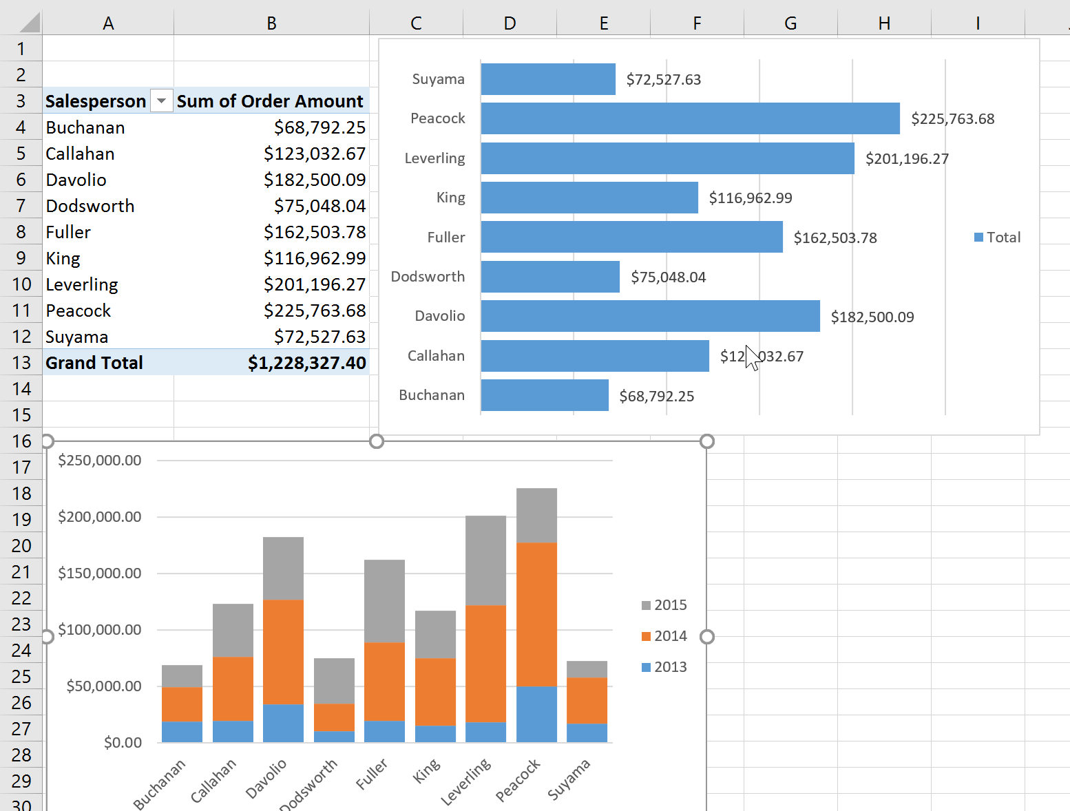
8 Let s insert a bar chart from our main dashboard Pivot Table. 1. Click within the Pivot Table >> Analyze >> PivotChart. In this example we ll insert a Bar chart. 2. We will turn off the bottom horizontal axis (the numbers are too big to all fit nicely). Click the Chart Elements button >> Axes >> Deselect Primary Horizontal. Also, turn the Title, and Legend off here as well. 3. Next, let s turn on data labels. This will display the amount right next to the bar. Click the Chart Elements button >> Data labels >> Outside End 4. Finally, increase the size of the bar by decreasing the gap to 25%. Right mouse click any data series bar >> Format data series >> Gap Width: 25% 8

9 9

10 % of Orders Salesperson per Country 10

11 Slicers Slicers allow you to filter your dashboard s data source in a visual way that is clear to understand. You can use slicers to quickly look at segments of your data, such as a fiscal year of information. Unlike a pivot table filter, you can see how one filter has affected the selections left available for other filters. So imagine you have two filters, Year and Type. When you slice out Expenses, you ll no longer be able to select any Expenses from any of the charts. This may sound simple, but it really makes for an easy to control Excel dashboard. 1. To insert a slicer, click the Dashboard worksheet tab. From the Analyze tab of the PivotChart Tools, Select insert Slicer. In this example we ll select Fund. Click OK. Your slicer is inserted. 2. The first thing we will do is connect this slicer to all of our PivotCharts (PivotTables). When we make a selection from the slicer we want it to filter out info on all of our PivotCharts (PivotTables). To do this, right mouse click the Slicer. OR from the Options tab of the Slicer, select Report Connections from the Slicer group. 3. Check the box to the left of each PivotTable you wish to connect it to. Click OK. To filter the info, simply click on one of the Funds listed. You can hold down your Control key to select various items from the Slicer list. 11

12 4. Use the Clear Filter option to clear the filter off of all of the charts. 5. To change the color of the slicer, use the Slicer Styles group of the Options tab. 6. To add more columns (instead of having it horizontal), use the Buttons group and the columns option. Use the corner handle to resize. 7. To insert your next slicer, repeat the steps. 8. Insert a Timeline, click within the PivotTable. From the Analyze Tabb >> Filter Group >> Insert Timeline. Select the date field (in this example, Order Date). Click OK. Please note, you will need to use the same steps as the 12

13 slider and connect the timeline to all of your PivotTables. 9. The timeline has an option to switch the date period to Years, Quarter, Months, Days. 13

14 PivotTable Tips & Tricks As soon as you create a new pivot table (or select the cell of an existing table in a worksheet), Excel displays the Options tab of the PivotTable Tools contextual tab. Among the many groups on this tab, you find the Show/Hide group that contains the following useful command buttons: Field List to hide and redisplay the PivotTable Field List task pane on the right side of the Worksheet area. +/- Buttons to hide and redisplay the expand (+) and collapse (-) buttons in front of particular Column Fields or Row Fields that enable you to temporarily remove and then redisplay their particular summarized values in the pivot table. Field Headers to hide and redisplay the fields assigned to the Column Labels and Row Labels in the pivot table. Format the Values in the PivotTable To format the summed values entered as the data items of the pivot table with an Excel number format, follow these steps: 1. Click the name of the field in the pivot table that contains the words "Sum of" and then click the Field Settings button in the Active Field group of the PivotTable Tools Analyze tab. Excel opens the Value Field Settings dialog box. You can also right mouse click the number in the actual PivotTable and select Value Field Settings. 2. Click the Number Format button in the Value Field Settings dialog box. The Format Cells dialog box appears with the Number tab displayed. 3. In the Category list, select the number format you want to assign. 4. (Optional) Modify any other options for the selected number format, such as Decimal Places, Symbol, and Negative Numbers. 5. Click OK two times to close both dialog boxes. 14

15 Filtering individual Column and Row fields The filter buttons attached to the Column and Row field labels let you filter out entries for particular groups and, in some cases, individual entries in the data source. To filter the summary data in the columns or rows of a pivot table, follow these steps: 1. Click the Column or Row field's filter button. 2. Deselect the check box for the (Select All) option at the top of the list box in the drop-down list. 3. Click the check boxes for all the groups or individual entries whose summed values you still want displayed in the pivot table. 4. Click OK. As with filtering a Report Filter field, Excel replaces the standard drop-down button icon for that Column or Report field with a cone-shaped filter icon, indicating that the field is currently being filtered and only some of its summary values are now displayed in the pivot table. To redisplay all the values for a filtered Column or Report field, you need to click its filter button and then click (Select All) at the top of its drop-down list. Then click OK. Sort a pivot table You can instantly reorder the summary values in a pivot table by sorting the table on one or more of its Column or Row fields. To sort a pivot table, follow these steps: 1. Click the filter button for the Column or Row field you want to sort. 2. Click either Sort A to Z or Sort Z to A at the top of the field's drop-down list. Click the Sort A to Z option when you want the table reordered by sorting the labels in the selected field alphabetically, from the smallest to largest numeric value, or from the oldest to newest date. Click the Sort Z to A option when you want the table reordered by sorting the labels in reverse alphabetical order (Z to A), values from the highest to smallest, and dates from the newest to oldest. You can also click in any data in the PivotTable and use the Sort and Filter options on the PivotTable Tools Ribbon. 15

16 Using Slicers to Filter PivotTables 1. Click any cell in the pivot table. Excel adds the PivotTable Tools contextual tab with the Analyze and Design tabs to the Ribbon. 2. On the PivotTable Tools Analyze tab, click the top of the Insert Slicer button in the Filter group. Excel opens the Insert Slicers dialog box with a list of all the fields in the active pivot table. 3. Select the check boxes for all the fields that you want to use in filtering the pivot table. Click OK. Excel will create a separate slicer for each of the selected fields. 4. After you create slicers for the pivot table, you can use them to filter its data simply by selecting the items you want displayed in each slicer. You select items in a slicer by clicking them just as you do cells in a worksheet hold down Ctrl as you click nonconsecutive items and Shift to select a series of sequential items. Modify the PivotTable Fields 1. From the Field List: a) To remove a field from the table, drag its field name out of any of the drop zones and, when the mouse pointer changes to an x, release the mouse button; or click its check box in the Choose Fields to Add to Report list to remove it its check mark. b) To move an existing field to a new place in the table, drag its field name from its current drop zone to a new zone at the bottom of the task pane. c) To add a field to the table, drag its field name from the Choose Fields to Add to Report list and drop the field in the desired drop zone note that if you want to add a field to the pivot table as an additional Row Labels field, you can also do this by simply selecting the field's check box in the Choose Fields to Add to Report list. Pivoting the table's fields As the name pivot implies, the fun of pivot tables is being able to restructure the table simply by rotating the Column and Row fields. In the PivotTable Field List pane, simply drag a label from the Row Labels drop zone to the Column Labels drop zone and vice versa so that the two field names are swapped. Voilà Excel rearranges the data in the pivot table at your request. 16

17 Modify the Summary Function By default, Excel 2013 uses the SUM function to create subtotals and grand totals for the numeric field(s) that you include in a pivot table. Some pivot tables, however, require the use of another summary function, such as AVERAGE or COUNT. To change the summary function that Excel uses in a pivot table, follow these steps: 1. Right-mouse click the field. Select a new summary function in the Value Field Settings dialog box. 2. Change the field's summary function to any of the following functions by selecting it in the Summarize Value Field By list box: Count to show the number of records for a particular category (note that Count is the default setting for any text fields that you use in a pivot table). Average to calculate the average (that is, the arithmetic mean) for the values in the field for the current category and page filter. Max to display the highest numeric value in that field for the current category and page filter. Min to display the lowest numeric value in that field for the current category and page filter. Product to multiply all the numeric values in that field for the current category and page filter (all non-numeric entries are ignored). Count Numbers to display the number of numeric values in that field for the current category and page filter (all nonnumeric entries are ignored). StdDev to display the standard deviation for the sample in that field for the current category and page filter. StdDevp to display the standard deviation for the population in that field for the current category and page filter. Var to display the variance for the sample in that field for the current category and page filter. Varp to display the variance for the population in that field for the current category and page filter. 3. Click OK. Excel applies the new function to the data present in the body of the pivot table. Conditional Formatting Excel 2013's conditional formatting lets you change the appearance of a cell based on its value or another cell's value. You specify certain conditions, and when those conditions are met, Excel applies the formatting that you choose. You might use conditional formatting to locate dates that meet a certain criteria (such as falling on a Saturday or Sunday), to call out the highest or lowest values in a range, or to indicate values that fall under, over, or between specified amounts. 17

18 1. Select the cells to which you want to apply conditional formatting. In some cases, you will select a single column or row of data in a table rather than an entire table. 2. On the Home tab, in the Styles group, click the Conditional Formatting button. A menu appears with several different options for specifying the criteria. 3. Point to Highlight Cell Rules and then select the type of criterion you want to use. Criteria options include Greater Than, Less Than, Between, Equal To, Text That Contains, A Date Occurring, and Duplicate Values. A window open where you can specify the values. 4. Enter the values you want reference in the text box (if necessary). Click the drop down arrow next to the format options and select the desired formatting. In the above example everything this is greater than will be a light red fill. 5. Click OK. 6. To clear the formatting, click Conditional Formatting (Home Tab, Styles group). Select Clear Rules >> Clear Rules from Entire Sheet. 18