Thermochronologic evidence for the exhumational history of the Alpi Apuane metamorphic core complex, northern Apennines, Italy

Transcription

1 Click Here for Full Article Thermochronologic evidence for the exhumational history of the Alpi Apuane metamorphic core complex, northern Apennines, Italy Maria Giuditta Fellin, 1,2 Peter W. Reiners, 3 Mark T. Brandon, 4 Eliane Wüthrich, 5 Maria Laura Balestrieri, 6 and Giancarlo Molli 7 Received 24 November 2006; revised 14 August 2007; accepted 29 August 2007; published 29 December [1] The Apennine Range is a young convergent orogen that formed over a retreating subduction zone. The Alpi Apuane massif in the northern Apennines exposes synorogenic metamorphic rocks, and provides information about exhumation processes associated with accretion and retreat. (U-Th)/He and fission-track ages on zircon and apatite are used to resolve exhumational histories for the Apuane metamorphic rocks and the structurally overlying, very low grade Macigno Formation. Stratigraphic, metamorphic, and thermochronologic data indicate that the Apuane rocks were structurally buried to km and 400 C at about 20 Ma. Exhumation to 240 C and 9 km depth (below sea level) occurred at Ma. By 5 Ma the Apuane rocks were exhumed to 70 C and 2 km. The Macigno and associated Tuscan nappe were also structurally buried and the Macigno reached its maximum depth of 7 km at 15 to 20 Ma. Stratigraphic evidence indicates that the Apennine wedge was submarine at this time. Thus we infer that initial exhumation of the Apuane was coeval with tectonic thickening higher in the wedge, as indicated by synchronous structural burial of the Tuscan nappe. From 6 to 4 Ma, thinning at shallow depth is indicated by continued differential exhumation between the Apuane and the Tuscan nappe at high rates. After 4 Ma, differential exhumation ceased and the Apuane and the Tuscan nappe were exhumed at similar rates (0.8 km/ma), which we attribute to erosion of the Apennines, following their emergence above sea level. Citation: Fellin, M. G., P. W. Reiners, M. T. Brandon, E. Wüthrich, M. L. Balestrieri, and G. Molli (2007), 1 Dipartimento di Scienze della Terra e Geologico-Ambientali, Università di Bologna, Bologna, Italy. 2 Now at Institut für Isotopengeologie und Mineralische Rohstoffe, ETH Zürich, Zurich, Switzerland. 3 Department of Geosciences, University of Arizona, Tucson, Arizona, USA. 4 Department of Geology and Geophysics, Yale University, New Haven, Connecticut, USA. 5 ETH Zürich, Geologisches Institut, Zurich, Switzerland. 6 Sezione di Firenze, IGG, Florence, Italy. 7 Dipartimento di Scienze della Terra, Università di Pisa, Pisa, Italy. Copyright 2007 by the American Geophysical Union /07/2006TC002085$12.00 TECTONICS, VOL. 26,, doi: /2006tc002085, 2007 Thermochronologic evidence for the exhumational history of the Alpi Apuane metamorphic core complex, northern Apennines, Italy, Tectonics, 26,, doi: /2006tc Introduction [2] The Apennine Mountains are the backbone of the Italian peninsula and separate the extensional, back-arc basin of the Tyrrhenian Sea to the west from the Adriatic foredeep to the east. The Apennine belt is underlain by a convergent orogenic wedge (Figure 1) that started at 30 Ma, and continued until at least 1 Ma. The orogen consists of a stack of east- and northeast-vergent thrust nappes (Figures 2 and 3), which have overridden and accreted foredeep sediments and basement rocks from the subducting Adriatic plate. An interesting feature of the Apennines is widespread extension directed normal to the orogen along its entire length (Figure 1). The Tyrrhenian Sea has formed by tectonic thinning associated with this synconvergent extension. The extension is also active along the entire west flank of the range, with the crest of the range marking the extensional deformation front. [3] The Apennine extensional domain includes several metamorphic complexes that form a structural culmination consisting of deeply exhumed metamorphic rocks. The largest and most deeply exhumed of these complexes is located at Alpi Apuane. The Alpi Apuane region is extremely rugged and has a maximum elevation of 1946 m. It is flanked by grabens to the east and west, which are filled with Plio-Pleistocene fluvio-lacustrine deposits. Exhumation of the Alpi Apuane core is attributed to slip on low-angle normal faults that mark the contact between the low-grade metamorphic units at the hanging wall, and the metamorphic core at the footwall. Tectonic thinning and erosion of the hanging-wall units may also contribute to the exhumation of the core. On the basis of these structural features, the Alpi Apuane can be defined as a metamorphic core complex [Malinverno and Ryan, 1986; Carmignani and Kligfield, 1990]. [4] Previous thermochronologic studies in this area [Abbate et al., 1994; Balestrieri et al., 2003] focused on apatite and zircon fission-track ages from the Apuane metamorphic complex. They show that the Apuane metamorphic rocks cooled from 240 to 110 C between 11 and 4 Ma, with an average exhumation rate of 0.7 km/ma. These authors attributed this cooling to the last stages of tectonic thinning and exhumation of the Apuane core. 1of22

2 Figure 1. Map of the Central Mediterranean region showing the major basins and surrounding mountain belts as well as the location of the Alpi Apuane. Black lines indicate major thrust fronts and arrows show the directions of extension and contraction [Jolivet and Faccenna, 2000]. [5] The Apennines-Tyrrhenian system is due to convergence between Africa and Eurasia, which produced several NW-dipping arcuate subduction zones and extensional basins in the Western Mediterranean (Figure 1) [e.g., Elter et al., 1975; Cherchi and Montardert, 1982; Dewey et al., 1989; Jolivet and Faccenna, 2000]. Several models have been proposed to explain extension in the Western Mediterranean, such as: (1) slab rollback [Malinverno and Ryan, 1986; Dewey, 1988; Royden, 1993; Cello and Mazzoli, 1996; Faccenna et al., 1996; Doglioni et al., 1998; Jolivet et al., 1998]; (2) postorogenic collapse [Carmignani and Kligfield, 1990; Carminati et al., 1998], and (3) slab detachment [Wortel and Spakman, 1992]. These models have assumed that the exhumation is mainly due to tectonic thinning. The nature of the tectonic thinning remains poorly understood, and the contribution of erosion, largely unknown. As an example, the island of Crete in the forearc of the retreating Hellenic subduction zone (Figure 1) exposes a low-angle normal fault that has juxtaposed highpressure/low-temperature (HP/LT) metamorphic rocks in the footwall, with carbonates in the hanging wall. The Cretan detachment was thought to be solely responsible for late Cenozoic exhumation of the HP/LT metamorphic rocks from a depth of 30 km. A study of metamorphic temperatures from above and below the Cretan detachment has demonstrated that the detachment fault accommodated only 5 to 7 km of the total exhumation and that the remain exhumation was caused by wholesale thinning of the overlying structural units [Rahl et al., 2005]. [6] Thus, to address the problem of exhumation of highgrade metamorphic rocks, it is necessary to constrain several fundamental questions regarding their structural evolution. In the Alpi Apuane case, these questions include the amount of section missing across bounding lithologic discontinuities that have been interpreted as normal faults [Carmignani and Kligfield, 1990; Carmignani et al., 1994], the depths and temperature conditions at which the inferred faults were active, and the detailed low-temperature thermal history of the Apuane core. [7] In this study we present new zircon and apatite (U-Th)/He (subsequently referred to as ZHe and AHe, respectively) and zircon and apatite fission-track (ZFT and AFT) results for the Alpi Apuane. These data elucidate several important elements of the structural evolution of the Apuane, including the timing, rate, and crustal depths at the time of slip on bounding faults. Our detailed reconstruction of the exhumation of the Alpi Apuane explains the role and spatial-temporal pattern of thickening versus thinning, and the role of extensional versus erosional exhumation in a retreating convergent orogen. We show that it is essential to study the thermal histories of both the metamorphic core and the structural cover to fully resolve the processes and history of exhumation. 2. Metamorphic and Structural Evolution [8] The northern Apennines formed by convergence of the Ligurian ocean and of the Adria-African plate [e.g., Vai and Martini, 2001]. The structurally highest thrust sheet of the northern Apennines is the Ligurian nappe, which is composed of Jurassic ophiolitic rocks and Jurassic to Paleogene sedimentary rocks. The Ligurian nappe represents the structural lid of the Apennine wedge. Southwestward subduction resulted in imbrication and accretion of thrust slices from the subducting Adriatic plate. The thrust nappes generally include Paleozoic basement, overlain by Mesozoic carbonates, and synorogenic foredeep sediments. The Ligurian nappe is overlain by the Epiligurian units, a sequence of middle Eocene to Pliocene sediments (Figures 2 and 3). These sediments are mainly shallow marine and indicate that the Apennines wedge formed below sea level, and only recently emerged as a subaerial thrust wedge [Zattin et al., 2002]. [9] The lowermost tectonic units of the northern Apennines consist of the moderate-pressure greenschistfacies metamorphic rocks of the Alpi Apuane. These units are predominantly Paleozoic basement [Pandeli et al., 1994, and references therein], covered by Mesozoic metalimestones, which in turn are capped by a turbidite unit, called the Pseudomacigno. The Pseudomacigno turbidites contain microfossils of Oligocene age [Dallan-Nardi, 1977; Montanari and Rossi, 1983] (Figure 4). The Alpi Apuane are surrounded and overlain by the Tuscan nappe, which experienced anchizonal metamorphic conditions [Reutter et al., 1983; Cerrina Feroni et al., 1983], and is itself overlain by the unmetamorphosed ophiolite-bearing Ligurian and Subligurian units (Figures 2, 3, and 4). [10] The Apuane metamorphic complex is divided into two units: the Massa unit to the west, and the Autoctono or Apuane unit to the east. The Massa unit consists mainly of Paleozoic crystalline basement covered by a Middle to Upper Triassic sedimentary sequence. The Apuane unit includes sedimentary units of Upper Triassic-to-Oligocene 2of22

3 Figure 2. (a) Topographic map of the northern Apennines. The square indicates the location of the geologic map reported in Figure 4. Metamorphic cores are: AP, Alpi Apuane; and MP, Monti Pisani. Main intramontane basins are: C, Casentino; G, Garfagnana; L, Lunigiana; M, Mugello; and S, Sarzana. (b) Simplified geologic map of the northern Apennines modified after Pini [1999]. age. These same sedimentary units are found in the overlying Tuscan nappe (Figure 4) but the metamorphic grade is much lower there. The Massa and Apuane units record different metamorphic conditions, but collectively they indicate increasing pressures and temperatures to the west. Peak P-T conditions determined from Fe-Mg chloritoid zoning in metapsammites in the Apuane unit are GPa and C; those in the Massa unit are GPa and C [Di Pisa et al., 1985; Franceschelli et al., 1986; Jolivet et al., 1998; Molli et al., 2000a, 2000b, 2002a]. Thus the Massa unit was buried to deeper levels (up to km) and now rests structurally above the Apuane unit. [11] The Tuscan nappe structurally overlies the Massa and Apuane units, and consists of a stratigraphic sequence of Upper Triassic to lower Miocene carbonates and greywackes that were detached from the crystalline basement and dismembered in a series of thrust sheets (Figure 4). The Upper Triassic to Eocene succession, which consists mainly of carbonates, is about 1.5 km thick [Decandia et al., 1968]. These are overlain by a 2- to 3-km-thick, upper Oligocene to lower Miocene siliciclastic succession called the Macigno 3of22

4 Figure 3. Tectono-stratigraphic diagram showing the stacking order of the main structural units in the northern Apennines modified after Cowan and Pini [2001]. Formation (Macigno) [Costa et al., 1992, and references therein]. Constraints on the burial history of the Tuscan nappe come from vitrinite reflectance of coaly inclusions [Reutter et al., 1983] and fission-track data on apatite [Abbate et al., 1994; Balestrieri, 2000; Zattin et al., 2002] and on zircon [Bernet, 2002] from the Macigno. These studies report quite different peak burial temperatures for the Macigno. Vitrinite reflectance data show a general pattern of high values near La Spezia (5.07% R m )onthe west, and values between 1.03 and 1.75% R m north of the Alpi Apuane, indicating peak burial temperature as high as C near La Spezia, and below 200 C north of the Alpi Apuane. In contrast, AFT ages indicate an increase of burial temperatures to the east with maximum burial temperatures of 125 C near La Spezia, and largely above 125 C in the Garfagnana area. ZFT ages are unreset and, therefore, suggest that the maximum burial temperature was lower than 200 C [Reiners and Brandon, 2006]. [12] K-Ar and 40 Ar/ 39 Ar dates on phengite in the Apuane metamorphic complex range from 27 to 11 Ma [Kligfield et al., 1986], thus burial under metamorphic conditions started soon after the Oligocene deposition of the now-metamorphosed Pseudomacigno unit. ZFT ages indicate that at 11 Ma, the Apuane core cooled through 240 C [Balestrieri et al., 2003], a temperature roughly coincident with the brittle-ductile transition of quartzitic rocks. K-Ar dates between 27 and 24 Ma have been related to the peak metamorphic conditions during the first polyphasic deformation event (D1 [Kligfield et al., 1986; Carmignani and Kligfield, 1990]). The D1 structures were redeformed during a later polyphasic D2 event, under ductile to brittle conditions, when kilometer-scale dome-like structures were produced [Carmignani et al., 1978; Carmignani and Giglia, 1979; Carmignani and Kligfield, 1990; Carmignani et al., 1994, and references therein]. The latest D2 stages are associated with high-angle strike-slip to extensional brittle faults [Ottria and Molli, 2000]. During the D1 event, a brecciated evaporite of probable Upper Triassic age at the base of the Tuscan unit (Calcare Cavernoso [Trevisan, 1962; Baldacci et al., 1967]) acted as a glide horizon, which was later reworked during the D2 event as a detachment fault complex [Carmignani and Kligfield, 1990]. According to fluid inclusion data, during the D2 event the brecciated fault zone was last active at a depth of about 10 km, assuming a paleogeothermal gradient of 31 C/km [Hodgkins and Stewart, 1994]. The Apuane D2 ductile structures have been interpreted in several strongly contrasting ways and have been related to both post-nappe refolding resulting from a continuous contractional history [Carmignani et al., 1978; Boccaletti et al., 1983; Cello and Mazzoli, 1996; Jolivet et al., 1998], and to kilometer-scale shear zones accommodating crustal extension [Carmignani and Kligfield, 1990; Carmignani et al., 1994; Storti, 1995]. [13] Previous fission-track work shows that the Alpi Apuane basement was exhumed to temperatures below 200 C between 5 and 2 Ma (Figure 5) [Abbate et al., 1994; Balestrieri et al., 2003]. At this time the thrust front of the northern Apennines was still actively propagating northeastward and it was located 100 km away from the modern Alpi Apuane. The modern topographic relief was also developed at this time, as recorded in the stratigraphy of tectonic depressions surrounding the Alpi Apuane, in the Lunigiana and Garfagnana region, and the Sarzana and Viareggio basins (Figure 2). The Viareggio basin is a tectonic depression with underlying basement as deep as 2.5 km [Mauffret et al., 1999] covered by marine sediments as old as upper Miocene [Bernini et al., 1990]. The adjacent Lunigiana, Garfagnana and Sarzana depressions are bor- 4of22

5 Figure 4. (a) Simplified geologic map of the Alpi Apuane. The location of the map is reported in Figure 2. (b) Simplified stratigraphic successions and of the Tuscan nappe and of Alpi Apuane metamorphic core modified after Decandia et al. [1968] and Carmignani et al. [2000]. dered by normal faults and are filled by continental deposits consisting of lacustrine clays of lower Pliocene age, covered by upper Pliocene alluvial conglomerates containing pebbles clearly derived from the metamorphic rocks of the Alpi Apuane [Bartolini and Bortolotti, 1971; Federici, 1973; Calistri, 1974; Federici and Rau, 1980; Bertoldi, 1988; Moretti, 1992; Bernini and Papani, 2002]. In continental basins throughout the northern Apennines, the end of the fluvio-lacustrine sedimentation and the beginning of predominantly fluviatile environments is thought to represent rapid uplift of the chain, which transgressed from west to east, beginning in the middle-upper Pliocene [e.g., Bernini et al., 1990; Bartole, 1995; Martini et al., 2001; Bartolini, 2003, and references therein]. [14] There is considerable uncertainty about the structures responsible for exhumation of the Alpi Apuane, the 5of22

6 Figure 5 6of22

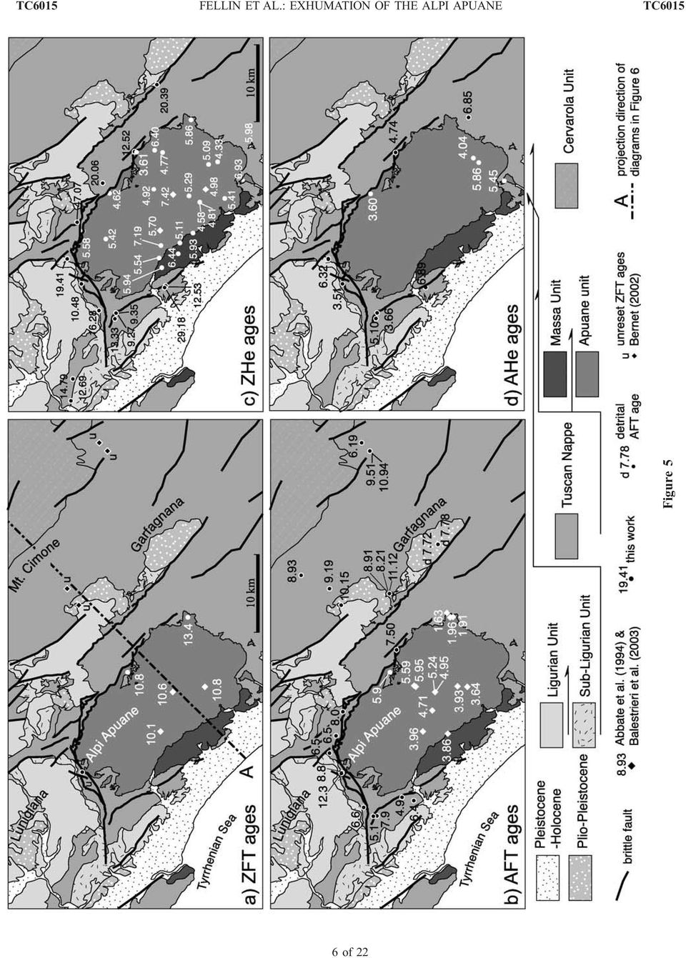
7 amount of throw on them at various crustal depths, and the relative roles of tectonic and erosional exhumation of the Alpi Apuane in the upper few kilometers of crust. The extensional faults bounding the upper Miocene-to- Pleistocene basins locally coincide with the shear zone bounding the Alpi Apuane [Carmignani et al., 1994; Ottria and Molli, 2000; Bernini and Papani, 2002]. Nevertheless, within the metamorphic core there is no evidence of significant offset in the brittle regime. Conflicting vitrinite reflectance and AFT data in the Tuscan nappe provide ambiguous constraints on the timing and depth of burial of this unit in and around the Alpi Apuane. Thus the amount of section missing across the shear zone separating the Alpi Apuane from the Tuscan nappe is largely unconstrained, as is the timing of its removal. For example, the shear zone may have been active only during the Miocene early D2 event, implying only erosional exhumation of the Alpi Apuane through the uppermost 10 km, or it may have been active as late as late Miocene and Pliocene, accommodating significant tectonic exhumation. In more general terms the question is: what is the role of extension versus erosion in the exhumation of the Alpi Apuane through various crustal depths? [15] These issues are important not only for understanding the Alpi Apuane itself, but also its role and significance in the larger northern Apennines orogen which, since the Miocene, has been affected by both extension in the hinterland and compression in the foreland of the belt [Carmignani and Kligfield, 1990; Carmignani et al., 1994; Keller et al., 1994; Storti, 1995; Jolivet et al., 1998, and references therein]. In this context, analysis of the orogenic evolution necessarily focuses on the transition from extension to compression, and specifically this paper aims to determine the time and depth at which extension was active in the Apuane, the most deeply exhumed and high relief part of the northern Apennines. 3. Low-Temperature Thermochronometry [16] New ZFT, AFT, ZHe, and AHe ages of samples from the Tuscan nappe and Alpi Apuane are shown in Tables 1 and 2. Here we provide only a brief description of the dating methods; details of analytical procedures are in Appendix A. The ZFT and AFT methods are based on measurements of the areal density of etched linear tracks produced by spontaneous fission of trace amounts of 238 U (see Wagner and Van den Haute [1992] for a summary). The fissiontrack ages refer to the time at which cooling below 240 C and 110 C occurred for zircon and for apatite, respectively (closure temperature T c ). Zircon and apatite (U-Th)/He chronometry is based on measurement of He produced by decay of U and Th. He diffusivity from crystals, analogous to fission-track annealing in some respects, is thought to be controlled by thermally activated volume diffusion. For typical cooling rates and crystal sizes, the effective (U-Th)/He closure temperatures for zircon and apatite are 180 C [Reiners et al., 2002, 2004] and 70 C [Farley, 2000], respectively. In cases of uniform and moderate to rapid cooling, (U-Th)/He ages are estimates of the time elapsed since cooling through a relatively narrow temperature range, the partial retention zone (PRZ) [Wolf et al., 1998]. Detrital crystals that never experienced temperatures above those of the PRZ show unreset or only partially reset ages. [17] New ZHe (36), AHe (11), AFT (12), and ZFT (3), ages of samples from the Tuscan nappe and Alpi Apuane are shown in Tables 1 and 2 and Figures 5 and 6. In the following discussion we integrate these data with previous AFT data from Abbate et al. [1994], Balestrieri [2000] and Balestrieri et al. [2003], and ZFT data by Bernet [2002] (Tables 3 and 4). Table 3 shows the details of AFT data whose ages were reported by Balestrieri [2000]. [18] All samples from the Tuscan nappe are from Oligocene to lower Miocene turbidites of the Macigno. AHe ages from the Macigno vary over a relatively narrow range between 3.5 and 6.9 Ma, AFT ages vary over the range between 4.9 and 12.3 Ma, whereas ZHe show a wide variation, between 9.3 and 47.1 Ma. Most of the Macigno ZHe ages fall between 9 and 16 Ma (Figures 5 and 6). However several of them overlap with or are considerably older than the estimated depositional age of the Macigno (20 28 Ma), suggesting that in some locations, the ZHe system in the Macigno has been only partially reset (Figure 7). This means that peak burial temperatures in at least some parts of the presently exposed Macigno in northwestern Tuscany did not significantly exceed 180 C. Because He ages of detrital grains resulting from partial resetting can vary widely, depending on protolith ages, it is difficult to constrain with certainty the age of cooling of the Macigno units as a whole, through the ZHe closure temperature of 180 C (or even if that temperature was reached during burial). Nevertheless, we tentatively interpret the abundant Ma ZHe ages in the Macigno near the Alpi Apuane as evidence for cooling through this temperature at approximately this time. This is consistent with an average AFT age of 8.2 ± 2.0 (1s)Mafor the Macigno samples in the region, as well as with AFT ages of detrital apatites (7.7 and 7.8 Ma) in Macigno cobbles from the Pliocene Barga fan (Table 3 and Figure 5). The latter evidence indicates that apatites in the Macigno cooled below 120 C at8 Ma, and by 3 4 Ma were already eroded and deposited in the Barga fan Figure 5. Geological sketch map of the Alpi Apuane and surroundings modified after Carmignani et al. [2000] and location of thermochronological data. (a) ZFT, zircon fission track; (b) AFT, apatite fission track; (c) ZHe, (U-Th)/He on zircon; and (d) AHe, (U-Th)/He on apatite. Circles indicate the location of data from this work, whereas diamonds show the location of data taken from previous studies. The black circles/diamonds are samples from the Tuscan nappe; the white circles/diamonds from the metamorphic units of the Alpi Apuane. 7of22

8 Table 1. Zircon and Apatite (U-Th)/He Data a Sample Unit Elevation, m Latitude, N Longitude, E U, mg Th, mg Raw Age, Ma FT Corrected Age, Ma est ± 2s, Ma Mass, mg mwar, mm U, ppm Th, ppm Th/U He, ncc/g Zircon (U-Th)/He 03AP33 Macigno Tuscan Nappe AP34 Macigno Tuscan Nappe AP46 Macigno Tuscan Nappe AP48 Macigno Tuscan Nappe AP55 Macigno Tuscan Nappe AP56 Macigno Tuscan Nappe GB07 Macigno Tuscan Nappe GB08 Macigno Tuscan Nappe GB09 Macigno Tuscan Nappe GB10 Macigno Tuscan Nappe RE20 Macigno Tuscan Nappe RE23 Macigno Tuscan Nappe Macigno Tuscan Nappe rep Macigno Tuscan Nappe AP47 Pseudomacigno Apuan AP58 Pseudomacigno Apuan GB04 Pseudomacigno Apuan GB06 Pseudomacigno Apuan GB12 Pseudomacigno Apuan RE21 Pseudomacigno Apuan RE22 Pseudomacigno Apuan RE24 Pseudomacigno Apuan FIO4z2 Pseudomacigno Apuan FO4A(4) b Pseudomacigno Apuan Pseudomacigno Apuan GB02 Hercynian Basement Apuan RE17 Hercynian Basement Apuan RE25A Hercynian Basement Apuan APUANE-1z2 Hercynian Basement Apuan APUANE-1z1 Hercynian Basement Apuan AP42 Hercynian Basement Apuan AP38 Met. Mesozoic succ. Massa Unit RE27 Hercynian Basment Massa Unit AP41 Hercynian Basement Massa Unit AP43 Hercynian Basement Massa Unit AP45 Hercynian Basement Massa Unit Apatite (U-Th)/He 03AP34 Macigno Tuscan Nappe GB07 Macigno/Tuscan Nappe GB09 Macigno Tuscan Nappe GB10 Macigno Tuscan Nappe RE20 Macigno Tuscan Nappe Macigno Tuscan Nappe AP51 Macigno Tuscan Nappe AP47 Pseudomacigno Apuan AP58 Pseudomacigno Apuan 03GB04 Pseudomacigno Apuan 03RE19 Pseudomacigno Apuan a Abbreviations: F T, a-ejection correction [Farley et al., 1996; Farley, 2002]; mwar, mass-weighted average radius (or simply radius for single grains). 8of22

9 Table 2. Zircon and Apatite Fission-Track Data a Zircon Fission Track Data Sample Unit Elevation, m Latitude, N Longitude, E Number of Grains rd, cm 2 Nd rs, cm 2 Ns ri, cm 2 Ni P(c 2 ), % Age, Ma ±2s Analyst z Value SM 2 Macigno Tuscan Nappe E E E D. Seward CN1 120 ± 5 FO4 Pseudomacigno Apuan E E E M. Bernet CN5 334 ± 3 MSV 2 Pseudomacigno Apuan E E E D. Seward CN1 120 ± 5 Apatite Fission Track Data Sample Unit Elevation, m Latitude, N Longitude, E Number of Grains rd, cm 2 Nd rs, cm 2 Ns ri, cm 2 Ni P(c 2 ), (%) Age (Ma) ±2s Analyst z Value CN5 03RE20 Macigno Tuscan Nappe E E E M.G. Fellin 355 ± 27 03GB07 Macigno Tuscan Nappe E E E M.G. Fellin 355 ± 27 SC 2 Macigno Tuscan Nappe E E E E. Wüthrich 277 ± 5 SC 5 Macigno Tuscan Nappe E E E b 1.4 E. Wüthrich 277 ± 5 S 1 Macigno Tuscan Nappe E E E E. Wüthrich 277 ± 5 S 3 Macigno Tuscan Nappe E E E E. Wüthrich 277 ± 5 S 4 Macigno Tuscan Nappe E E E E. Wüthrich 277 ± 5 SM 3 Macigno Tuscan Nappe E E E E. Wüthrich 277 ± 5 SM 4 Macigno Tuscan Nappe E E E E. Wüthrich 277 ± 5 SU 1 Macigno Tuscan Nappe E E E E. Wüthrich 277 ± 5 SU 2 Macigno Tuscan Nappe E E E E. Wüthrich 277 ± 5 MSV 2 Pseudomacigno Apuan E E E E. Wüthrich 277 ± 5 a Abbreviations: r d, induced track density in external detector adjacent to dosimetry glass (tracks cm 2 ); Nd, number of tracks counted on external detector adjacent to dosimetry glass; rs, spontaneous track density (tracks cm 2 ); N s, number of spontaneous tracks counted; r i, induced track density in external detector (tracks cm 2 2 ); N i, number of induced tracks counted; P (c) is (c)2 probability [Galbraith, 1981; Green, 1981]; age, the sample central fission-track age [Galbraith and Laslett, 1993] calculated using zeta calibration method [Hurford, 1990] and dosimetry glass CN5 for apatites, CN5 or CN1 for zircons. 9of22

10 Figure 6. Diagrams showing age-elevation data projected along a vertical plane, SW NE trending (for location, see Figure 5). The diagrams show the lack of age-elevation relationship within samples (a) from the Tuscan nappe (Macigno) and (b) from the Alpi Apuane. [Balestrieri, 2000]. All previously dated ZFT samples from the Macigno are clearly unreset [Bernet, 2002] as well as a new ZFT sample lying just north of the Alpi Apuane. [19] New ZFT, AFT, ZHe and four AHe ages from the Alpi Apuane are shown, along with earlier data, in Figures 5 and 6. Samples from the Alpi Apuane were collected in the Massa and Apuane units (in particular in the Paleozoic phyllites and metavolcaniclastics), and in the Oligocene metagraywackes (Pseudomacigno). The paucity of suitable apatite crystals in most lithologies of the Alpi Apuane limited the number of AHe analyses that we could perform. Nearly all ZHe, AFT and AHe ages vary over a relatively narrow range of 4 7 Ma whereas ZFT ages vary between 10 and 13 Ma. ZHe ages average 5.5 ± 0.9 Ma throughout the entire Alpi Apuane, and are in general slightly older than or the same as AFT ages [4.8 ± 0.9] in the Alpi Apuane 10 of 22

11 Table 3. Apatite Fission-Track Data From Balestrieri [2000] a s.d., mm Mean Confined FTL, mm Number of Confined Age, Ma ±1s Longitude, E r s,cm 2 N s r i,cm 2 N i S/I E, % Latitude, N Elevation, m Sample Unit GOM1 Macigno Tuscan Nappe E E / ± GOM2 Macigno Tuscan Nappe E E / ± GOM3 Macigno Tuscan Nappe E E / CAS1 Macigno Tuscan Nappe E E / ± CAS2 Macigno Tuscan Nappe E E / ± CAS3 Macigno Tuscan Nappe E E / CAST1 Macigno Tuscan Nappe E E / ± CAST2 Macigno Tuscan Nappe E E / CAST3 Macigno Tuscan Nappe E E / ± BARG1 sed. Plio-Pleistocene E E / ± BARG2 sed. Plio-Pleistocene E E / ± a Samples dated using the population method. Abbreviations: r s (ri), spontaneous (induced) track density; Ns (Ni), spontaneous (induced) counted tracks; S/I, number of analyzed crystals for spontaneous (S) and induced (I) track density determination; E%, the propagation of relative standard errors of the spontaneous and induced track counts; FTL, fission-track lengths; s.d., standard deviation of the confined track length distribution. core. The exception to this is one region in the extreme eastern corner of the Alpi Apuane, where AFT ages are as young as Ma. [20] Projection of ages onto an orogen-normal, SW NE transect shows no consistent relationship between ages and topography or horizontal distance within the Alpi Apuane, although the youngest ages are generally found in the easternmost Alpi Apuane (Figure 6). Similarly, no obvious relationships between age and topography or horizontal distance are observed for any chronometer outside the Alpi Apuane, in the Macigno (Figure 6). Most notably, however, there is a clear distinction between both ZHe and AFT ages in the Alpi Apuane and in the Macigno: within the Alpi Apuane, ZHe ages average 5.5 ± 0.9 Ma and AFT ages 4.8 ± 0.9 Ma; in the outlying Macigno, most ZHe ages are 9 20 Ma, and AFT ages average 8.2 ± 2.0 Ma (Figures 5 and 6). This indicates that the Alpi Apuane core cooled through temperatures of 180 C and 120 C about 4 Ma later than the overlying Macigno. The sharp ZHe age contrast of 4 to 14 Ma within a few hundred meters across the inferred detachment on the northeast side of the Alpi Apuane (Figure 5) also indicates that this structure was active through depths corresponding to temperatures as low as 180 C. Finally, the similarity of AHe ages in both the Alpi Apuane core and the overlying Macigno suggests that final exhumation through the upper 2 3 km was not accomplished via tectonic exhumation, but via erosion Thermal Modeling Thermal Profile of the Crust [21] In order to derive exhumation rates, closure depths, and temperatures from thermochronometric data, it is necessary to estimate the thermal field during exhumation. We use a simplified analysis here, based on a one-dimensional steady-state solution for a single uniform crustal layer with a specified basal temperature (details are given by Brandon et al. [1998] and Reiners and Brandon [2006]). The temperature T ( C) as a function of depth z (km) is represented by TðÞ¼T z s þ T L T s þ H T L 1 expð _ez=k Þ _e 1 expð _el=k Þ H T z _e ; where _e (km/ma) is the erosion rate, L (km) layer thickness, k (km 2 /Ma) thermal diffusivity, H T ( C/Ma) parameter of internal heat production, T S surface temperature, and T L basal temperature at z = L. The use of a uniform and steady thermal model is clearly an approximation, but this approach seems warranted given that the thermal histories of the samples are mainly influenced by the structure of the thermal field at a regional scale. Batt and Brandon [2002] compared this one-dimensional solution to a more complete two-dimensional thermal-kinematic solution for a wedge. They concluded that the one-dimensional solution provides a good approximation for relating low-temperature cooling ages to exhumation rates. The following factors account for why this approximation works: (1) The presence of a subduction zone and accretion at the base of the wedge tends to maintain a constant basal temperature, consistent ð1þ 11 of 22

12 Table 4. Published Thermochronologic Data From the Alpi Apuane Sample Unit Elevation, m Latitude, N Longitude, E AFT Age, Ma AFT ± 1s ZFT Age, Ma ZFT - 2s ZFT + 2s ZHe Age, Ma Z He ± 2s Source GOM1 Macigno Tuscan Nappe unreset Bernet [2002] GOM3 Macigno Tuscan Nappe unreset Bernet [2002] CAS2 Macigno Tuscan Nappe unreset Bernet [2002] CAS3 Macigno Tuscan Nappe unreset Bernet [2002] AR1 Pseudomacigno Apuan Abbate et al. [1994] AR2(4) Pseudomacigno Apuan (AR2A) a AR3 Pseudomacigno Apuan FC3 Pseudomacigno Apuan FC5 Pseudomacigno Apuan FO1 Pseudomacigno Apuan FO4 Pseudomacigno Apuan FO5 Pseudomacigno Apuan CP1 Hercynian Basement Apuan CP3(4) Hercynian Basement (CIP3/CIP3A) a Apuan G2 Hercynian Basement Apuan G3(4) (G3A) a Hercynian Basement Apuan MD1 (MAD1) Hercynian Basement Massa Unit Abbate et al. [1994]; Balestrieri et al. [2003] Abbate et al. [1994]; Balestrieri et al. [2003] Abbate et al. [1994] Abbate et al. [1994] Abbate et al. [1994] Abbate et al. [1994] Abbate et al. [1994] Abbate et al. [1994] Abbate et al. [1994]; Balestrieri et al. [2003] Abbate et al. [1994] Balestrieri et al. [2003] Abbate et al. [1994] a Multigrain aliquot, with number of crystals given in parentheses. 12 of 22

13 Figure 7. Frequency histogram of (U-Th)/He ages on zircons (ZHe) from the Tuscan nappe (Macigno). ZHe ages from this unit are only partially reset indicating maximum burial temperatures of 200 C. with the assumption of a constant T L in equation (1). (2) The vertical gradients in the thermal field are much greater than those in the horizontal, even in cases where horizontal velocities are large [Batt and Brandon, 2002]. As a consequence, one can commonly ignore the horizontal dimension in the thermal field. (3) Low-temperature thermochronometers, such as (U-Th)/He and fission-track systems, are mainly sensitive to the shallowest part of the thermal field (70 to 240 C), which adjusts rapidly to changes in the surface boundary condition, and is relatively insensitive to the basal boundary condition. As a result, the relevant closure isotherms will tend to closely follow the depth predicted by a steady state solution ( quasi steady state ). In contrast, 40 Ar/ 39 Ar thermochronometers have much higher closure temperature (200 to 500 C) and are more strongly affected by the full thermal field and by transients in exhumation rates. (See discussion by Reiners and Brandon [2006] about the sensitivity of thermochronometers to transients.) [22] The solid line in Figure 8 shows the estimated steady state thermal profile for no exhumation, where _e = 0 in (1). The surface temperature T S is set to 14 C, which is the present mean-annual temperature at sea level in the northern Apennines. The thermal diffusivity is set to k = 27.4 km 2 /Ma (0.87 mm 2 /s), based on local measurements by Pasquale et al. [1997] and general compilations by Beardsmore and Cull [2001] and Clauser and Huenges [1995]. Temperatures near the base of our model are constrained by the peak metamorphic conditions recorded by the Apuane metamorphic complex. These units were accreted before the onset of exhumation and thus are representative of the maximum temperatures and depths within the Apennine wedge. PT estimates for the Apuane unit are C, and GPa, and for the Massa unit, C, and GPa [Di Pisa et al., 1985; Franceschelli et al., 1986; Jolivet et al., 1998; Molli et al., 2000a, 2000b, 2002a]. These pressures are equivalent to depths of 15 to 22 km, and 22 to 30 km, respectively (assuming an average crustal density of 2750 kg/m 3 ). We use the modern surface heat flow in the Po Basin, which is 40 mw/m 2 (equivalent to a surface thermal gradient of 20 C/km) [Della Vedova et al., 2001], to represent the _e = 0 case. Surface heat flow is greater in the Apennines, reaching a maximum of 70 to 90 mw/m 2, but these values are influenced by fast erosion within the mountain range. On the basis of these constraints, we estimate that the parameter for the internal heat production H T is 4.5 C/Ma (equal to a volumetric heat production of 0.3 mw/m 3 ) and that T L = 540 CatL = 30 km. The dashed lines show the steady state temperature profile as a function of different erosion rates. Exhumation causes a steeper Figure 8. Thermal profiles for the Massa and Apuane units based on a one-dimensional steady state solution [Reiners and Brandon, 2006]. For details see text (section 2.1.1). H T, heat production parameter; T L, basal temperature of layer L; k, thermal diffusivity; T s, surface temperature; dt/dz, surface thermal gradient; PRZ, partial retention zone. Grey bars indicate the partial retention zone for 40 Ar/ 39 Ar ages for muscovite as estimated by Reiners and Brandon [2006]. 13 of 22

14 Figure 9. Schematic illustration of the effect of topographic relief on the isotherm at depth: z is the depth of the isotherm with respect to elevation; h is the difference between a sample elevation and the local mean average elevation; z m is the depth of the isotherm with respect to the local mean elevation; and s is the difference between the closure depth of a sample and the mean closure depth. The closure depths and erosion rates of each sample derived from a steady state solution for no topographic relief [Brandon et al., 1998; Reiners and Brandon, 2006] are corrected for the relief of topography (h) and of closure depth (s). thermal gradient near the Earth s surface. As a result, isotherms will be closer to the surface, but cooling rates will be faster as well. We need to consider both of these effects when estimating effective closure temperature for each of our thermochronometers Exhumation Rates [23] We estimate exhumation rates using the method given by Brandon et al. [1998] and Reiners and Brandon [2006]. This calculation finds a steady value for _e that agrees with the observed cooling age, the one-dimensional thermal model (as parameterized above), and the effective closure temperature, as given by the Dodson equation, which is a function of cooling rate and the diffusion parameters for the relevant thermochronometer. This approach allows us to compare exhumation rates determined by different thermochronometers. We note that this approach can break down if exhumation rates changed rapidly while the thermochronometers were moving through their respective closure isotherms. The cooling ages, together with stratigraphic and metamorphic evidence, can be used to detect if large transients have occurred. [24] On the basis of ages of all four systems, the steady model estimates effective closure depths of km for AHe, km for AFT, km for ZHe and km for ZFT. These results refer to conditions where there is no topographic relief. Local surface topography (relief) can produce topography on the closure isotherm [Stüwe et al., 1994; Mancktelow and Grasemann, 1997; Braun, 2002]. Figure 9 shows how we can account for this phenomenon. The thermal solution given by equation (1) provides a reliable estimate of the depth of the closure isotherm relative to the local mean elevation. Thus the influence of surface topography on isotherm topography can be accounted separately by calculating how variations h around the local mean elevation are relative to variations s around the local mean depth of the closure isotherm. This problem is easily solved by downward continuation of the surface thermal field [e.g., Turcotte and Schubert, 2002; Braun, 2002]. We have developed a Fourier-based method for this calculation (M. Brandon, work in progress, 2007). We used modern topography to estimate h and then calculated s for the steady-state closure isotherm. Our estimated closure depths and exhumation rates have all been corrected to account for the full vertical distance at the sample locality z = z m + h s, as measured from the closure isotherm to the surface (Figure 9). This correction is generally small for our data here, with (h s)/z m < 10 percent for all but four samples. [25] Using maximum and minimum ages for each thermochronometer, we have derived model curves of exhumation rate as a function of time (Figure 10). For the Alpi Apuane, these results indicate increasing exhumation rates (from to 0.8 >1.4 km/ma) in the late Miocene, followed by decreasing rates (to 0.6 km/ma) in the early Pliocene. A relatively wide range of exhumation rate is permitted by the large variation in ages for any given system, but the data show a clear increase in exhumation rates to at least as high as 1.4 km/ma in the late Miocene, followed by a decrease after about 5 Ma, to values 0.6 km/ma. For the Macigno, the results show exhumation rates between 0.3 and 0.8 km/ma from middle Miocene through Pliocene. Thus, in the Macigno, none of the thermochronometric systems shows significant changes in exhumation rate from middle Miocene through Pliocene, and they are all consistent with cooling of the Macigno below 180 C at or after Ma. After the Pliocene, low exhumation rates of the Macigno are suggested by the occurrence in the upper Pliocene deposits of the Barga fan of detrital AFT ages of 7 8 Ma (see Table 3). These detrital ages from Macigno cobbles are similar to the AFT ages of the presently exposed Macigno in Garfagnana and around the Alpi Apuane. Thus the cooling ages of the presently exposed Macigno are similar to the Macigno cooling ages that were eroded during Pliocene, and this suggests that after Pliocene time the Macigno in this area has not been significantly eroded. [26] The exhumation paths for the Alpi Apuane and the Macigno are schematically summarized by the timeelevation diagram in Figure 11, illustrating that between 7 and 4 Ma the Alpi Apuane were rapidly exhumed at very shallow depths whereas at the same time the Tuscan nappe was exhumed at a constant rate Combining Thermochronometric and Geological Data [27] In order to more directly compare the cooling paths of the Tuscan nappe (Macigno) and the Alpi Apuane metamorphic core, we measured ZHe ages of two samples 14 of 22

15 Figure 10. (a, b) Diagrams showing the exhumation rates derived for different thermochronometers from cooling ages through the Dodson relation and a steady-state solution for the advective heat flow problem with ages corrected for topographic effects [Brandon et al., 1998; Reiners and Brandon, 2006]. Gray regions envelope the results obtained for each thermochronometer for surface thermal gradient between 20 C/km and 30 C/km in the case of a steady state advection. (c, d) Diagrams show the envelopes of the erosion rates. They show that in the Alpi Apuane peak exhumation rates of 0.8 >1.4 km/ma occur between 7 and 4 Ma, whereas in the Tuscan nappe (Macigno) exhumation rates are constantly below 0.8 km/ma. ( and 03RE20) collected within 300 m, on opposite sides of a 10-m-thick, NE-dipping brittle shear zone with an inclination angle of (Figures 5 and 11), suspected of being a major detachment responsible for much of the unroofing of the Apuane core [Molli et al., 2002b]. The Pseudomacigno of the metamorphic core in the footwall of this structure, yielded a ZHe age of 3.6 ± 0.3 Ma, whereas the Macigno in the hanging wall yielded a ZHe age of 12.5 ± 1 Ma, which may be only a partially reset age. A similar age contrast is also observed from analogously paired samples on the western side of the Alpi Apuane: the Macigno near Carrara shows partially reset ZHe ages of 29.2 ± 2.3 and 12.5 ± 1.0 Ma, whereas ZHe ages in the Massa unit range between 5.9 ± 0.5 and 6.4 ± 0.5 Ma (Figure 5). [28] Time-depth paths of the Alpi Apuane and of the Macigno suggest different depths until 4 Ma on the northern and western sides, and perhaps until as late as 2 Ma on the easternmost side, where the youngest AFT ages are found. The rough trend of gradually decreasing ZHe, AFT, and AHe ages from west to east across the Apuane (Figure 6) suggests that this depth difference was 15 of 22

16 Figure 11. (a) Time-closure depth diagram: closure depths (z) for each thermochronometer have been determined from cooling ages through the Dodson relation and a steady state solution for the advective heat flow problem with ages corrected for topographic effects [Brandon et al., 1998; Reiners and Brandon, 2006]. (b) Sketch map of the study area with the location of the topographic profile A and of two samples collected at the opposite walls of a main extensional ductile-brittle shear zone. (c) Schematic model showing a possible mechanism of exhumation of the Alpi Apuane over the last 6 Ma based on the time-depth diagram reported in Figure 11a. Cooling data constrain a temperature gap of about 130 C from 7 to 4 5 Ma between the Alpi Apuane and the overlying Macigno, corresponding to a total thickness removed of 3 4 km assuming the thermal parameters shown in Figure 8. After 4 5 Ma the Alpi Apuane and the Macigno were exhumed as a single body. Part of the thickness removed consists of the Mesozoic succession, 1.5 km thick [Decandia et al., 1968], which lies below the Macigno, and the remaining 2-km-thick section is indicated in the sketch model as?missing section. 16 of 22

17 removed progressively from west to east (Figure 11). The contrasting exhumation paths of the Alpi Apuane core and its cover (Figure 11) suggest that the removal of a crustal thickness of the order of 3.6 ± 0.5 km must have occurred along the Apuane detachment under brittle conditions (at temperatures lower than 200 C) between 6 and 4 Ma. Since 4 Ma, the two units, already resting at very shallow levels, reached the surface, probably via erosion, as a single coherent body. [29] The schematic structural interpretation that accommodates these thermochronometric requirements is based on constraints on the geometry of significant faults in and around the Alpi Apuane. The geometry of the faults that accommodated removal of this section can be estimated not only from local exposures but also from structural, borehole and seismic data in the northern Apennines. The fault zone bounding the Apuane core shows a variable attitude with a moderate (45 ) to low inclination angle (Figure 5). On the western side of the Alpi Apuane, the Macigno is in direct contact with the basal unit of the Tuscan nappe (Calcare Cavernoso) through a high-angle, SW-dipping fault zone. On the eastern side of the Apuane, although there is evidence of brittle, NE-dipping normal faults dissecting the Tuscan nappe, vertical throws on individual structures are likely less than a few hundred meters. The mainly carbonate Mesozoic succession stratigraphically below the Macigno is up to 1.5 km thick [Decandia et al., 1968], and it could represent a significant portion of the removed section. The rest of the removed section, here named the missing section (see Figure 11), could have been partly eroded from above the Alpi Apuane and could now rest below the Tuscan nappe. This missing section would be 2.1 km thick. Further constraints come from the presence of extensional faults dissecting the Alpi Apuane [Carmignani et al., 1994; Ottria and Molli, 2000; Molli et al., 2002b], and bounding the Pliocene-to-Pleistocene basins around the Alpi Apuane [Moretti, 1992; Bernini and Papani, 2002]. Maximum estimates of the vertical offsets related to the main faults bordering these basins are 2.5 km [Bernini and Papani, 2002]. Seismic and borehole data show that these basins are asymmetric grabens with low angle, NE-dipping, master faults and antithetic, steep SW-dipping faults. This fault system is detached on the basement top [Bernini and Papani, 2002; Argnani et al., 2003]. In the internal northern Apennines the basement top lies at a depth of 3 4 km, to the NWof the Alpi Apuane, and this shows that at a large scale the basement top dips away from the Apuane high with a moderate inclination angle. All these data provide constraints on how after 5 Ma high-to-low angle brittle faults may have interacted with or dissected the Apuane detachment, which at that time was being exhumed at a very shallow depth. A synthesis of these considerations, which facilitates the exhumational histories required by the thermochronometric data and is consistent with surficial geology, is shown in Figure 11. [30] Further constraints on the restoration of the geometry of the Apuane detachment are provided by the presence of pebbles derived from the Apuane metamorphic core in the fluvio-lacustrine sediments of upper Pliocene age in Garfagnana and Lunigiana [Calistri, 1974; Moretti, 1992]. These observations require that at 3 Ma, a portion of the Alpi Apuane core was already exposed to erosion while local regions were still at depths corresponding to temperatures above C (e.g., the SE corner of the metamorphic core where 2 Ma AFT ages are found). Our attempt to restore the brittle activity of the Apuane detachment is shown in Figure 11. The model is based on the aforementioned constraints and two basic assumptions: a surface geothermal gradient of 20 C/km and the lack of thermal perturbations related to relief until 5 Ma. The lack of thermal perturbations is supported by the fact that during Pliocene-to-lower Pleistocene the northern Apennines were characterized by a low relief with scattered lacustrine basins [Bartolini, 2003] Thermochronometric Versus Fluid Inclusion Data [31] Hodgkins and Stewart [1994] estimated trapping conditions of fluid inclusions from the brecciated metamorphic rocks at the highest structural level within the Alpi Apuane, concluding that minimum trapping temperatures were C, and suggesting that the Apuane detachment was last active at a depth of about 10 km. Other studies based on vein and fluid compositions [Costagliola et al., 1998, 1999] concluded that hydrothermal circulation at shallow levels (below C) in the Alpi Apuane was essentially absent. Our thermochronometric evidence shows that the brittle fault zone exposed along the eastern margin of the Alpi Apuane was active under brittle conditions, at temperatures below 200 C. This suggests that at temperatures higher than 200 C, hydrothermal activity resulting in vein deposition in the Alpi Apuane was restricted to a few areas, and does not provide a constraint on the final depths of fault motion and exhumation of the core. We suggest that the quartz and calcite veins observed in the Alpi Apuane do not constrain the last activity of the Apuane detachment fault but are likely associated with earlier stages of development of the fault zone and/or with the D2 folding event. 4. Conclusions 4.1. Extension Versus Erosion [32] The combined results from all four thermochronometric systems in the Alpi Apuane core and overlying Tuscan nappe (Macigno Formation) have allowed us to reconstruct and compare the different exhumation paths of these two units at temperatures below 240 C. ZFT ages are Ma in the Alpi Apuane core, and are unreset in the surrounding Macigno. ZHe ages of 25 samples from the Alpi Apuane core average 5.5 ± 0.9 Ma, and show a possible younging trend toward the east. These 5.5 Ma ages are significantly younger than ZHe ages of the overlying Macigno, the youngest of which are 9 16 Ma. Some ages in the Macigno are much older than 9 16 Ma and only partially reset, suggesting burial temperatures did not significantly exceed 180 C. AFT and AHe ages within the Alpi Apuane core are indistinguishable from one another, averaging 4.8 ± 0.9 Ma for AFT and 4.7 ± 1.1 Ma for AHe. 17 of 22

18 Figure 12. Time-depth paths of the Alpi Apuane (Apuane unit and Massa unit) and of the overlying Tuscan nappe (Macigno) obtained from thermochronometric data presented in this work integrated with Ar/Ar [Kligfield et al., 1986] and peak metamorphic conditions data [Di Pisa et al., 1985; Franceschelli et al., 1986; Jolivet et al., 1998; Molli et al., 2000a, 2000b, 2002a]. Low-temperature thermochronometric data indicate that high exhumation rates in the Alpi Apuane can be interpreted as related to events of tectonic exhumation whereas low exhumation rates can be related at least during the last 4Ma mainly to erosional exhumation. AFT ages in the Macigno average 8.2 ± 2.0 Ma, significantly older than in the Alpi Apuane core, whereas AHe ages in the Macigno average 5.3 ± 1.4 Ma essentially the same as in the Alpi Apuane core (though possibly slightly older) (Figure 12). [33] Our cooling ages indicate an exhumation rate increase of the Alpi Apuane core in the late Miocene from km/ma to >1.4 km/ma, followed by a decrease 0.6 km/ma in the Pliocene (Figure 10). The only inconsistency to this interpretation is exhumation rates inferred to be as high as 1.7 km/ma in a small region in the easternmost Alpi Apuane. Unlike the exhumation history of the Alpi Apuane core, cooling data in the surrounding and overlying Tuscan nappe records almost constant exhumation at 0.8 km/ma through the late Miocene to the Pliocene. The higher exhumation rates of the Alpi Apuane core in the late Miocene-early Pliocene imply that the tectonic boundary between these two units was active as an extensional brittle fault accommodating 3.6 ± 0.5 km of tectonic unroofing of the Alpi Apuane core. After this, the Alpi Apuane core and the Tuscan nappe were exhumed as a single body. The presence of pebbles from the Alpi Apuane core in the early Pliocene Garfagnana, Val di Vara and Sarzana intramontane basins indicate that at 2 4 Ma the Alpi Apuane core rocks were at the surface. [34] Our reconstruction is consistent with interpretations of seismic and stratigraphic data in the onshore and offshore basins of western Tuscany [e.g., Bernini et al., 1990; Bartole, 1995; Martini et al., 2001; Bartolini, 2003; Argnani et al., 2003, and references therein]. These seismic and stratigraphic data indicate that the main extensional faults bordering the basins of northwestern Tuscany were active during the late Miocene early Pliocene, locally with minor vertical throws during the late Pliocene, and that finally during the late Pliocene early Pleistocene both this area and a much larger portion of the northern Apennines experienced regional uplift and erosion. [35] Finally, our data show that during the late Pliocene the exposure of the Apuane massif was coincident with the end of extensional exhumation and the onset of erosional exhumation. This result suggests that erosion is largely responsible for the present elevation of the Apuane massif and for its domal shape Thickening Versus Thinning [36] Our results bracket metamorphism and ductile deformation of the Alpi Apuane to be after Ma and before Ma (ZFT ages). This age bracket is after deposition of the Pseudomacigno and before cooling below the ZFT closure temperature (240 C). These ages are largely compatible with previous 40 Ar/ 39 Ar ages measured on phengite that range between 27 and 11 Ma [Kligfield et al., 1986]. The 40 Ar/ 39 Ar data were obtained from powdered specimens that impede an unequivocal distinction 18 of 22

19 between crystalization and cooling age of the dated mineral. Our ZFT ages suggest that the younger 40 Ar/ 39 Ar ages most likely record cooling of the Alpi Apuane massif implying that the peak metamorphism dates back to the early-middle Miocene (20 Ma). [37] The thermochronometric data document an apparent decrease of the exhumation rate in the Alpi Apuane core at about 11 Ma (Figure 12). The decrease could be due to the uncertainties related to the 40 Ar/ 39 Ar data that show a wide range of variation, and to the paucity of the available ZFT ages. On the other hand, the Alpi Apuane experienced significantly varying exhumation rates with the highest rates occurring during extensional denudation under ductile and brittle conditions. [38] The extensional denudation of the Alpi Apuane has been long debated as it is a key for the understanding of exhumation processes of deep metamorphic rocks in a convergent orogen above a retreating subduction zone. Extension in the Alpi Apuane has been interpreted as related to either underplating and thickening in the internal northern Apennines [Carmignani et al., 1978; Boccaletti et al., 1983; Cello and Mazzoli, 1996; Jolivet et al., 1998], or crustal thinning leading to formation of the northern Tyrrhenian Sea and collapse of the Apennines [Carmignani and Kligfield, 1990; Carmignani et al., 1994; Storti, 1995]. The distinction between thickening versus thinning and extensional versus erosional exhumation, and the relative timing of each, are essential because these processes migrate through time and space with the accretionary wedge and its back-arc basin, in response to subduction zone retreat. The thermochronologic data indicate that the initial exhumation of the Alpi Apuane (from a depth range of km to <9 km) occurred before Ma, that is before the late Miocene when sedimentation first occurred in the Viareggio basin [Bernini et al., 1990; Mauffret et al., 1999]. The formation of the Viareggio basin relates to the onset of crustal thinning in this sector of the Tyrrhenian Sea and of the Apennines. This suggests that the initial exhumation of the Alpi Apuane occurred before the formation of the adjacent extensional basins. [39] Data from the hanging wall of the Apuane detachment provide further evidence on the timing of thickening versus thinning processes. The key observations from the hanging wall of the Apuane detachment are: (1) after deposition, the Macigno was structurally buried by overthrusting higher units (the Subligurian, Ligurian and Epiligurian units; Figure 3); (2) the peak burial temperature in the Macigno greywackes did not significantly exceed the ZHe Tc, that corresponds to a maximum burial depth of 7 km; (3) the reset ZHe ages cluster around Ma and the younger reset ages are 9 10 Ma old; (4) the reset ZHe are interpreted to indicate cooling of the Macigno at Ma. Our observations suggest that cooling in this sector of the Tuscan nappe did not begin before Ma. At Ma the Alpi Apuane core had already exhumed to shallow depth (<9 km). At this time, the Apennines were still submerged as indicated by the presence of the Epiligurian units that are middle Eocene to Pliocene shallow-marine sediments deposited above the Apennine wedge. Thus structural burial of the Tuscan nappe and initial exhumation of the Alpi Apuane core occurred at the same time and before Ma in conditions of no sub-aerial erosion. This coincidence in timing suggests that the initial exhumation of the Alpi Apuane core occurred when there was no erosion and contraction was still operating in the internal Apennines both at shallow and deep crustal levels. Between 6 and 4 Ma the differential exhumation at shallow crustal levels of the metamorphic core and its hanging wall occurred at the same time with formation of extensional basins around the Alpi Apuane and with ongoing contraction at the front of the Apennines wedge. After 4 Ma, no differential exhumation is recorded and unroofing is mainly driven by erosion Exhumation of High-Grade Metamorphic Rocks: The Alpi Apuane and the Crete Cases [40] The exhumation of the Alpi Apuane is in many ways similar to the exhumation of the high-grade metamorphic rocks of Crete, which is the fore-high arc of the Hellenic retreating subduction zone [Jolivet et al., 1996; Thomson et al., 1999; Rahl et al., 2005, and references therein]. The similarities comprise (1) the role of erosion, (2) the exhumation of the hanging wall units and (3) their brittle deformation. (1) In both cases erosion played no role in the initial exhumation as this occurred before the onset of topographic relief. Erosion played an important role in the Alpi Apuane only at very shallow depth in the last 2 4 Ma as they uplifted and formed the most prominent relief in the northern Apennines. (2) During initial exhumation from deep to shallow crustal levels, the hanging wall units of both the Apuane and the Cretan detachments remained at shallow depth confined in the upper 7 km of the crust. (3) During exhumation at shallow depth (<10 km) brittle stretching affected mostly the hanging wall units. [41] Another striking similarity is that in both cases the wealth of available data still fails to explain fully the exhumation of the high-grade metamorphic rocks from deep (20 30 km) to shallow (10 km) crustal levels. Nevertheless, our data from the Alpi Apuane indicate that the exhumation at deep crustal levels is more likely related to thickening and accretion. Similarly, the exhumation at high rates of the Cretan high-grade metamorphic rocks from deep to shallow crustal levels could be more likely explained by contractional processes. Appendix A: Analytical Procedures for Age Determinations A1. Fission-Track Analysis [42] Sample preparation for the AFT and ZFT analysis consists of three main procedures: separation, etching and irradiation. Apatites and zircons were separated from 5 kg bulk samples using standard heavy liquids (Li-metatungstate and methylene iodide) and magnetic separation techniques. [43] On samples reported in Table 2, zircon and apatite fission-track central ages (±2s [Gailbraith and Laslett, 19 of 22

20 1993]) were measured and calculated using the externaldetector and the zeta-calibration methods with IUGS age standards [Hurford, 1990]. Spontaneous tracks were revealed through polishing of grain mounts and etching. Different etching conditions were used by analysts for apatites and zircons, and samples were irradiated with thermal neutrons at different reactors. Apatite grain mounts by M. G. Fellin were etched with 5N HNO 3 at 20 C for 20 s, and were irradiated with thermal neutrons in the O.S.U. Triga reactor (USA) with a nominal neutron fluence of ncm 2. Apatite grain mounts by E. Wüthrich were etched in 7% HNO 3 at 21 C for 50 s and were irradiated at ANSTO facility, Lucas Heights (Australia) with a total integrated requested flux of ncm 2. On zircons spontaneous tracks were revealed through polishing of grain mounts and etching in a eutectic mixture of KOH and NaOH at 210 C for hours. Zircon samples by D. Seward were irradiated at ANSTO facility, Lucas Heights (Australia) with a total integrated requested flux of ncm 2. The zircon sample by M. Bernet was irradiated at the O.S.U. Triga reactor (USA) with a normal fluence of n cm 2. After irradiation, for all samples a standard glass CN-5 or CN-1 (Table 3) was used as a dosimeter to measure neutron fluence, and induced fission tracks in the low-u muscovite, which cover apatite grain mounts and glass dosimeters, were etched in 40% HF at 20 C for 40 min. [44] Samples by Balestrieri [2000] reported in Table 3 were dated using the population method. Two aliquots of apatite (for spontaneous and induced track counting) from each sample were mounted in epoxy resin, polished and etched with 5% HNO 3 at 20 C. Irradiation was performed in the Lazy Susan facility (Cd ratio 6.4 for Au and 48 for Co) of the reactor Triga Mark II of the University of Pavia. Neutron fluence is ncm 2. Parameters used for age calculation are s = cm 2 ; l = a 1, l F = a 1. Track counting was performed using a Leica Orthoplan microscope at 1250x magnification. Lengths were measured with a Leica Microvid stage. A2. (U-Th)/He Analysis [45] Zircon and apatite (U-Th)/He ages were measured on single grains (with the exception of four multi-crystal aliquots denoted in Table 1), and performed by Nd:YAG laser heating for He extraction and sector inductively coupled plasma mass spectrometry (ICP-MS) for U-Th determinations at Yale University. He was measured by 3 He isotope dilution using a quadrupole mass spectrometer following cryogenic purification. Uranium and Th were measured by 229 Th and 233 U isotope dilution using a Finnigan Element2 inductively coupled plasma mass spectrometer. The a-ejection was corrected using the zircon method described by Farley [2002]. Estimated 2s uncertainty is 8% for zircon He ages, and 6% for apatite He ages. [46] Dated crystals were hand-picked from separates with high power (160) stereo-zoom microscopes with cross polarization for screening inclusions, although most of these zircon crystals did contain small (5 20 um) visible inclusions. Selected crystals were measured and digitally photographed in at least two different orientations for a-ejection corrections. Crystals were loaded into 1-mm Pt foil tubes, which were then loaded into copper or stainless steel sample planchets with sample slots. Planchets were loaded into a 10-cm laser cell with sapphire window, connected by high-vacuum flexhose to the He extraction/ measurement line. Once in the laser cell and pumped to < torr, crystal-bearing foil tubes were individually heated using power levels of 1 5 W on the Nd:YAG, for 3 min for apatite or 20 min for zircon. Temperatures of heated foil packets were not measured, but from experiments relating luminosity and step-wise degassing of both apatite and zircon, we estimate typical heating temperatures of 950 C for apatite, and C for zircon. [47] Acknowledgments. This work was supported by the RETREAT project, funded by grant EAR from the NSF Continental Dynamics program to M. T. Brandon and P. W. Reiners. Diane Seward is acknowledged for her collaboration providing additional data for this work and reviewing an early version of the paper. The authors are grateful to Massimiliano Zattin for his help in the sample collection, for constructive suggestions, and for his overall contribution to this work. References Abbate, E., M. L. Balestrieri, G. Bigazzi, P. Norelli, and C. Quercioli (1994), Fission-track datings and recent rapid denudation in northern Apennines, Italy, Mem. Soc. Geol. Ital., 48, Argnani, A., G. Barbacini, M. Bernini, F. Cimurri, M. Ghielmi, G. Papani, F. Rizzino, S. Rogledi, and L. Torelli (2003), Gravity tectonics driver by Quaternary uplift in the northern Apennines: Insights from the La Spezia-Reggio Emilia geo-transect, Quat. Int., , Baldacci,F.,P.Elter,E.Giannini,G.Giglia,A.Lazzarotto, R. Nardi, and M. Tongiorgi (1967), Nuove osservazioni sul problema della Falda Toscana e sulle interpretazioni dei flysch arenarei tipo Macigno dell Appennino settentrionale, Mem. Soc. Geol. Ital., 6, Balestrieri, M. L. (2000), Exhumation ages and blockfaulting on the eastern flank of the Serchio graben (northern Apennines), paper presented at 9th International Conference on Fission Track Dating and Thermochronology, Univ. of Melbourne Fission Track Res. Group, Lorne, Victoria, Australia. Balestrieri, M. L., M. Bernet, M. T. Brandon, V. Picotti, P. W. Reiners, and M. Zattin (2003), Pliocene and Pleistocene exhumation and uplift of two key areas of the northern Apennines, Quat. Int., , Bartole, R. (1995), The North Tyrrhenian-northern Apennines post-collisional system: Constraints for a geodynamic model, Terra Nova, 7, Bartolini, C. (2003), When did the northern Apennine become a mountain chain?, Quat. Int., , Bartolini, C., and V. Bortolotti (1971), Studi di geomorfologiaeneotettonica.i-idepositicontinentali dell Alta Garfagnana in relazione alla tettonica Plio-Pleistocenica, Mem. Soc. Geol. Ital., 10, Batt, G. E., and M. T. Brandon (2002), Lateral thinking: 2 D interpretation of thermochronology in convergent orogenic settings, Tectonophysics, 349, Beardsmore, G. R., and J. P. Cull (2001), Crustal heat flow: A guide to measurement and modeling, 324 pp., Cambridge Univ. Press, Cambridge, U. K. Bernet, M. (2002), Exhuming the Alps through time: Clues from detrital zircon fission-track ages, Ph.D. dissertation, 135 pp., Yale Univ., New Haven, Conn. Bernini, M., and G. Papani (2002), La distensione della fossa tettonica della Lunigiana nord-occidentale (con Carta geologica alla scala 1:50.000), Boll. Soc. Geol. Ital., 121, Bernini, M., M. Boccaletti, G. Moratti, G. Papani, F. Sani, and L. Torelli (1990), Episodi compressivi neogenico-quaternari nell area estensionale tirrenica nord-orientale. Dati in mare e a terra, Mem. Soc. Geol. Ital., 45, Bertoldi, R. (1988), Una sequenza palinologica di età rusciniana nei sedimenti lacustri basali del bacino di 20 of 22