A Progress Report on Business Cycle Models

Transcription

1 Federal Reserve Bank of Minneapolis Quarterly Review Vol. 18, No. 4, Fall 1994 A Progress Report on Business Cycle Models Ellen R. McGrattan* Economist Research Department Federal Reserve Bank of Minneapolis The views expressed herein are those of the author and not necessarily those of the Federal Reserve Bank of Minneapolis or the Federal Reserve System.

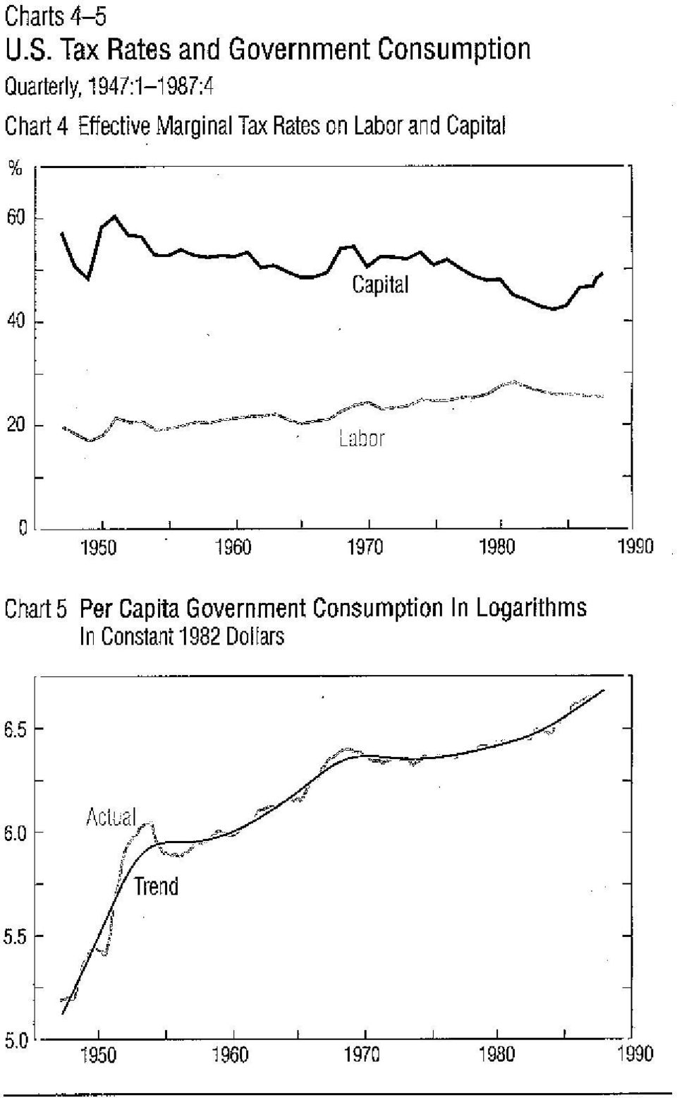
2 Before using a specific model to analyze economic data or policies, economists must have confidence that the model will fit the data along certain dimensions. One of the goals of modern business cycle research has been to develop economic models that mimic the cyclical patterns of aggregate data such as gross national product, its components, and labor market aggregates, like employment and hours. A natural starting point for assessing the progress made toward this goal is the Kydland and Prescott (1982) model. This business cycle model, which is widely regarded as the standard, assumes that fluctuations are driven by technology shocks. As a first cut, it has done remarkably well. However, certain failures of the model have led to subsequent research. Early attempts to extend the Kydland-Prescott model, such as the Hansen (1985) model, have been partially successful, but recent work by Chang (1992), Braun (1994), McGrattan (1994a), and others looks more promising. Their findings suggest that adding fiscal shocks to the basic Kydland-Prescott model can significantly improve its ability to mimic the data. The critical assumption of the Kydland-Prescott model is that technology shocks are the main source of aggregate fluctuations. When simulated, this model displays cyclical behavior similar to that of U.S. data. Specifically, the Kydland-Prescott model can account for much of the variability in gross national product, and it can correctly predict that consumption is less variable than income, while investment is more variable. But this model predicts a variability of consumption, hours worked, and productivity that is too low relative to the data and a correlation between productivity and hours worked that is too high. Hansen (1985) has noted the failures of the standard Kydland-Prescott model and suggests that they may be due to the way the labor choice is modeled. Kydland and Prescott assume that individuals choose a certain number of hours per week to work. Hansen makes that choice an either/or decision: Individuals work either a set number of hours per week or no hours at all. By making labor indivisible, Hansen has created a model that is better able to mimic the variability of total hours worked than is the Kydland-Prescott model. But Hansen s model cannot capture the observed variability in consumption and productivity and the low correlation between productivity and hours worked. So, while altering the labor choice appears to be a good solution, it leaves several problems unresolved. Recently, a different extension of the Kydland-Prescott model has been proposed by Chang (1992), Braun (1994), McGrattan (1994a), and others. These researchers note that the standard Kydland-Prescott model ignores fiscal shocks, which are an important source of aggregate fluctuations. They therefore add fiscal shocks (such as changes in tax rates and government consumption) to the standard model to see if the model can then better mimic the variability in consumption, hours worked, and productivity as well as the observed near-zero correlation between productivity and hours worked. It can. Why? Because households alter their investment and labor decisions in response to changes in tax rates: they substitute between taxable and nontaxable activities and thereby affect the variability of consumption, hours worked, investment, and output. Here, I begin with an examination of the U.S. data patterns. Then, after describing a version of the standard Kydland-Prescott model, an extension by Hansen, and an extension by Braun (1994) and others, I compare the predictions of all three to the data. Patterns in the Data Since the goal of business cycle studies is to account for fluctuations in the aggregate data, examining these data for the United States before trying to construct models to explain them seems logical. In this section, I describe the general patterns of gross national product (GNP), its components, and hours worked; then I present several specific series of the tax rates on labor and capital and government consumption. Gross National Product and Its Components... I plot quarterly GNP in constant 1982 dollars for the post World War II sample in Chart 1. Along with GNP, I plot a trend that captures the low frequencies of this series. Since business cycle theories are being used to explain the higher frequencies, many researchers focus their attention on the difference between the actual and trend series. For GNP, the maximum deviation is around 6 percent. The sample begins with the post World War II recession, followed by an increase in output due to the Korean War. Other large deviations occur at the end of the sample during the time of the oil crises and during the Reagan years. Chart 2 presents the ratios of the major components of GNP (private and government consumption and investment) to GNP itself. The levels of and variations in the components of GNP should be comparable to the data analogues. In this chart, private consumption is the ratio of consumer nondurables plus services to GNP, investment is the ratio of fixed investment plus consumer durables to GNP, and government consumption is the ratio of government purchases to GNP. For the postwar sample, private consumption averages 54 percent of GNP, investment averages 23 percent of GNP, and government consumption averages 22 percent of GNP. The remaining 1 percent is attributable to net exports and inventories. Regarding the cyclical behavior of these series, note that private consumption is less volatile than investment and that the ratio of government consumption to GNP varies considerably over the sample. The most striking periods are the war years. Around 1950, government consumption greatly increased because of the Korean War, and in the late 1960s and early 1970s, it increased because of the Vietnam War. In Chart 3, I plot deviations from trend of GNP and total hours worked (both in logarithms). Notice that the percentage deviation for the two is similar in magnitude. Notice also that the two are positively correlated. If the same plot is made for capital stock, another factor of production, the deviations are much smaller relative to output.... And Fiscal Variables Models with fiscal variables also consider tax rates and government consumption. In Chart 4, I plot measures of the effective marginal tax rates on labor and capital income. The tax series are constructed using Joines (1981) definition. He uses data on income reported in the Statistics of Income (IRS, various years) to determine the proportion of income that is attributable to capital and the proportion that is attributable to labor. He then computes estimates of effective marginal tax rates on these factor incomes. (See Joines 1981 for details and McGrattan 1994a, Appendix A, for the estimates used in these plots.) Other researchers have constructed different measures for tax rates. For example, Barro and Sakahasul (1986) re-

3 port estimates of the average marginal tax rates from the U.S. federal individual income tax returns for Their estimates are averages of tax rates listed in the income tax schedule, and their series has the same cyclical pattern as the series in Chart 4, but it has a higher mean and a higher growth rate over the sample. Seater (1985) uses a definition that is similar to Joines (1981) to obtain a measure of the effective marginal tax rate on income due to federal taxes. Again, its cyclical pattern is the same as that of the series in Chart 4, but it has a lower mean. For the tax on capital, Judd (1992) computes a rate that has very different properties than the rate computed by Joines definition. (See Chart 4.) In Judd s case, the tax rate is approximately white noise, which is a sequence of uncorrelated random variables. I argue later in the paper (and in Appendix A) that the choice of process for the rate has important implications for the effect of capital taxes on aggregate fluctuations. If the tax rate on capital is white noise, then the variation in output and employment due to capital taxes is zero. In Chart 5, I plot quarterly government consumption in constant 1982 dollars and its trend for the post World War II period. This plot shows that movements in the ratio of government consumption to GNP (in Chart 2) are not due solely to movements in GNP. As in the case of the tax rates of Chart 4, government consumption fluctuates significantly and the series is highly serially correlated. Also, the effects of shocks to government consumption depend crucially on how persistent the changes are. The Standard Model s Predictions... As is common in most modern business cycle studies, I begin with Kydland and Prescott s 1982 model. In this section, I describe a variant of that standard model (similar to the one described in Prescott 1986) to illustrate what the model can and cannot do well. The model economy is populated by a large number of identical households that make consumption, investment, and labor decisions over time. Each household s objective is to choose sequences of consumption, {c t } t=0, and hours of leisure, {l t } t=0, that maximize expected discounted utility: (1) E[ t=0 βt u(c t,l t ) x 0 ] where x 0 denotes the initial conditions that the household takes as given when forming expectations and β (such that 0 < β< 1) is the subjective discount factor. The households maximize utility subject to several constraints. The first is their budget constraint, (2) c t + i t r t k t +w t n t which states that expenditures in time period t on private consumption goods, c t, and investment goods, i t, cannot exceed the household s income. Households have two sources of income. One is the income from renting capital to firms. By period t, the capital stock that has accumulated is k t ; the rental income is r t k t. The other source of income is wage income. Households allocate one unit of time between leisure or work. The fraction of that one unit of time spent on leisure activities is l t and the fraction spent on work is n t. If the household earns w t per unit of time worked in t, then w t n t is its wage income. A second constraint for the household is the following capital accumulation equation. I assume that capital in the next period is equal to new investment plus what remains after depreciation: (3) k t+1 = (1 δ)k t + i t where δ is the rate of depreciation. The initial capital stock, k 0, is assumed to be known to the households. That is, k 0 is one element of the vector x 0 in equation (1). In this model, households behave competitively and take prices of inputs as given. Therefore, in terms of their budget constraint in period t in (2), households take the prices, r t and w t, as given. These variables, which are indexed by t, are assumed to be known to the household prior to making decisions in period t. To make their optimization problem well posed, I assume that when households form expectations, they know the relationship between the economy s state and the prices. To derive this relationship, I next describe the firms. Here, firms operate in competitive markets and therefore take prices as given when solving their own constrained maximization problem. Each firm s objective in period t is to maximize profits (where some given production technology is assumed); that is, (4) max κt,η t y t r t κ t w t η t subject to (5) y t = λ t f(κ t,η t ) where κ t is the per capita capital stock and η t is the per capita number of hours worked in period t. The firm sells y t goods, where the price per unit is equal to one. The cost of the capital and labor inputs is equal to r t κ t + w t η t, where r t and w t are taken as given by the firm. Output of the firm depends not only on capital and labor inputs but also on the level of technology λ t. For example, new inventions or discoveries would lead to higher levels of technology. The firm optimally chooses capital and labor so that marginal products are equal to the price per unit of input; that is, (6) r t = λ t [ f(κ t,η t )/ κ t ] (7) w t = λ t [ f(κ t,η t )/ η t ]. Given the expressions for the rental and wage rates in (6) and (7), I can define the state of the economy as (κ t, λ t ). Note that I have not included per capita hours worked in this list of state variables for a simple reason. If prices are functions of κ t and λ t, then the decisions of an individual household are functions of κ t, λ t, and its own capital stock, k t. Thus the number of hours that the household works is given by some function, n t = n(k t,κ t,λ t ). Assuming that households are identical implies that k t = κ t and that η t can be written as a function of κ t and λ t ; that is, η t = η(κ t,λ t )=n(κ t,κ t,λ t ). Substituting the per capita hours worked function into the marginal conditions for the firm implies that factor prices can be written as functions of κ t and λ t. That is, prices can be written as functions of the proposed state vector. To complete the description of the household s problem, I must specify a process for technology, which is the only source of fluctuations in the standard model. I as-

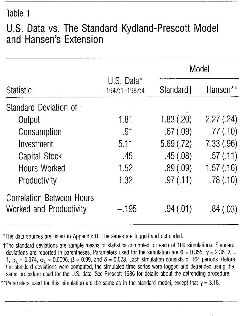
4 sume that the process for technology is a first-order autoregressive process, (8) λ t+1 = (1 ρ λ ) λ + ρ λ λ t + ε λ,t+1 where 1 < ρ λ < 1 and ε λ,t is a serially uncorrelated variable drawn from a normal distribution with mean 0 and variance σ 2 λ. 1 The decision making of the household can now be summarized by a well-posed constrained optimization problem. This problem can be stated as follows: Choose c t = c(κ t,λ t ), i t = i(κ t,λ t ), and n t = n(κ t,λ t ) that maximize (1), with x 0 =(k 0,λ 0,κ 0 ), subject to the following constraints: (9) c t + i t r t k t + w t n t (10) l t =1 n t (11) κ t+1 = h(κ t,λ t ) (12) η t = η(κ t,λ t ) and subject to the capital accumulation equation in (3), the price functions in (6) and (7), the law of motion for the exogenous state in (8), the law of motion for per capita capital stock h (which is assumed to be known), and the function that relates the states and the per capita hours worked η (which is also assumed to be known). An equilibrium for this economy is a set of decision functions for the household, c(k t,κ t,λ t ), i(k t,κ t,λ t ), and n(k t,κ t,λ t ); a set of decision functions for the firm, κ(κ t,λ t ), η(κ t,λ t ), and y(κ t,λ t ); pricing functions, r(κ t,λ t ) and w(κ t,λ t ); and a law of motion for per capita capital stock, κ t+1 = h(κ t,λ t ), such that the following hold true: The household s decision functions are optimal given the pricing functions and the law of motion for per capita capital stock. The firm s decision functions are optimal given the pricing functions; that is, they satisfy (6) and (7). Markets clear for labor, capital, and goods; that is, (13) n(κ t,κ t,λ t )=η(κ t,λ t ) (14) κ t = κ(κ t,λ t ) (15) c(κ t,κ t,λ t )+i(κ t,κ t,λ t )=y(κ t,λ t ). Expectations are rational; that is, (16) h(κ t,λ t ) = (1 δ)κ t + i(κ t,κ t,λ t ). One of Kydland and Prescott s (1982) objectives was to quantify the responses of output, consumption, investment, and hours worked to technology shocks. To mimic their calculations, I must choose functional forms for utility, u( ), and production, f( ), to parameterize the model and to compute the equilibrium decision functions of the household. Kydland and Prescott (1982) describe a method that can be used to approximate the decision functions. Their approximation yields a linear relationship between each decision variable and the capital stock and technology shock. Here, I use their method of approximation. 2 For utility and production, I choose (17) u(c,l) = log(c) + γlog(l) (18) f(k,n)=k θ n 1 θ. Therefore, the parameters of the model are the parameters for the technology shock, ( λ,ρ λ,σ λ ), the discount factor, β, the depreciation rate, δ, the weight on leisure in utility, γ, and capital s share of income, θ. Since the mean of the technology shock only affects the scale of output, consumption, investment, and the capital stock, I set λ =1. To obtain the coefficient on technology, ρ λ, in (8), I construct a least-squares estimate by regressing λ t on its lagged value. The time series for the technology shock is taken to be λ t = y t /(k θ tn 1 t θ ). Since the trend in technology is positive, the trend must be removed. This is done by regressing the logarithm of the technology shock [log(λ t )] on a constant and a time trend and subtracting the estimated trend. For the variance of ε t, I use the variance from the data, namely, σ λ = (I match correlations of the model series with those in the data after logging and detrending both, using the detrending method from Prescott 1986.) I set the discount factor, β, equal to A value of 0.99 implies an average annual interest rate of 4 percent. To get an estimate of the depreciation rate, δ, I project i t (k t+1 k t )onk t.the least-squares estimate is I choose the capital s share of income, θ, and the weight on leisure in utility, γ, so that the sample means of the data and the model are equated. 3 The data that I use to determine θ and γ are the capital/output ratio and hours worked as a fraction of total hours available. I also use the estimates for β and δ. For output, I use the sum of private consumption and investment, since this model assumes that output does not include government consumption. The average level of the capital/output ratio over the sample is If I use Hill s (1985) estimate of 1,134 hours per quarter of discretionary time, then the average fraction of work time over the sample is From these estimates, I calculate a value of for θ, which is approximately equal to [1 β(1 δ)]/β times the capital/output ratio. The estimate of γ is (1 θ)(1/n 1) (1 δk/y), which is equal to 2.36, where n is the fraction of work time and k/y is the capital/output ratio. Now that I have a specification for the utility and production functions and parameters, the model can be simulated. I begin by generating a realization for the stochastic process {ε λ,t } of length T. With the sequence (ε λ,t,t= 1,2,...,T), I can generate a sequence of technology shocks, given some initial value λ 0. The sequence of technology shocks, along with an initial condition for the capital stock, can then be used in conjunction with the decision functions to generate sequences for k t,c t,i t,n t,and y t. In Table 1, I report the results from simulating the standard model. If statistics for U.S. data (in the first column) are compared to statistics for the standard model (in the second column), these numbers suggest that the standard model can account for the observed variability in output, investment, and capital stock. For example, the standard deviation of output is 1.81 in the data and 1.83, on average, for the simulated time series. The main failures of the model are its inability to generate the observed variability in consumption, hours worked, and productivity and its inability to generate a near-zero correlation between hours worked and productivity. The standard deviation of consumption is only 0.67 percent for the standard model; it is 0.91 percent for the data. For hours worked, the model only captures 60 percent of the observed variability: the model predicts a standard deviation of 0.89 percent while

5 the data shows a deviation of 1.52 percent. As a result, productivity (which is defined as output per hour of work) varies too little in the simulations.... Improve Slightly With Indivisible Labor... Hansen (1985) notes the failures of the Kydland-Prescott model to explain key labor statistics and suggests that they may be due to the way the labor choice is modeled. Because the standard model fails to capture certain key features of the U.S. labor market series, Hansen (1985) considers the following extension. He assumes that households can work a fixed number of hours, N, or none at all. In the aggregate, his model predicts that a certain fraction of the workforce is employed for N hours per period and a certain fraction is unemployed. As I show later, this assumption implies a greater elasticity of labor than that of the standard model. To avoid problems with nonconvexities, Hansen (1985) redefines the household s choice set in terms of lotteries, following Rogerson (1988). A lottery is the probability of working, and a contract between households and firms is the probability of working N hours and not the number of hours worked. Suppose that the utility function defined over consumption and leisure takes a logarithmic form; for example, u(c,l) = log(c) +Alog(l) for A > 0. Then the expected utility in period t is given by log(c t ) + Alog(1 N)α t, where α t is the probability in period t of working N hours. In the aggregate, α t of the households work N hours and 1 α t work 0 hours. Thus the per capita hours worked is given by n t = Nα t. The optimization problem can therefore be specified, as in the previous section, with (19) u(c,l) = log(c) + γl where γ = log(1 N)/N. Compare (19) with (17). Because leisure enters linearly in (19), there will be more substitution between leisure at different dates in Hansen s model. With greater substitution, the model should predict higher variability in leisure and hours worked. In the third column of Table 1, I report the results of simulating the Hansen model with the utility function defined in (19) [rather than (17)]. The parameters used in simulating this model remain the same as in the previous section, with one exception. The weight on leisure, γ, in (19) must be set equal to 3.18 in order to match the capital/output ratio and the fraction of work time for the data and the model. Because labor supply is more elastic, the variability of the indivisible-labor model is greater than that of the divisible-labor model (that is, the standard model). Note, in particular, that the number of hours worked in Hansen s model has a standard deviation of 1.57, which is almost twice that of the standard model. But Hansen s more accurate approximation of hours worked comes at the expense of his figures for output and investment, which are too variable. In Hansen s model, the standard deviation for output is 2.27 percent, which is 25 percent higher than that of the data; the standard deviation for investment is 7.33 percent in Hansen s model, which is 43 percent higher than that of the data. Hansen s model also does not significantly improve the predictions for the variability of consumption and productivity. The standard deviation of consumption is only 0.77 percent, which is significantly lower than the deviation of 0.91 percent observed in the data. And the standard deviation of productivity is only 0.78 percent, which is significantly lower than the deviation of 1.32 percent observed in the data and the deviation of 0.97 percent predicted by the standard model. Finally, Hansen s model does not predict the near-zero correlation between hours worked and productivity. As in the standard model, his prediction of 0.84 is too high. This result is affected by technology shocks, which only shift the labor demand schedule. If the labor supply schedule is fixed, then movements in the labor demand schedule generate a positive correlation between hours worked and real wages, which is equal to productivity.... And Significantly With Fiscal Shocks While the Hansen extension better matches the variability in hours worked found in U.S. data, it fails to substantively improve the standard Kydland-Prescott model. Chang (1992), Braun (1994), and McGrattan (1994a) are among the researchers who have noted that most of the failures of the standard model can be reconciled once fiscal shocks are included in the model. These researchers show that fiscal shocks can better mimic the observed patterns of aggregate fluctuations such as the variability in consumption, hours worked, and productivity and the near-zero correlation between hours worked and productivity. They also show that households significantly alter their investment and labor decisions in response to changes in tax rates. Households substitute between taxable activities and nontaxable activities and, in doing so, affect the variability of output, consumption, investment, hours worked, and productivity. Changes in government consumption can also affect the volatility of these variables since an increase in government consumption must be financed by taxes, and taxes induce changes in investment and employment. Furthermore, changes in fiscal variables lead to changes in households labor supply, and these changes offset technologically induced changes in firms labor demand. Thus the correlation between hours worked and productivity is not as high as the standard model predicts. 4 Consider the following changes to the models discussed in the previous two sections. Assume that preferences can depend on government consumption: (20) E[ t=0 βt u(c t +πg t,l t ) x 0 ] where 0 < β < 1. The weight of government consumption in utility, π, depends on the relative value of private consumption, c t, and public consumption, g t. If π = 1, then private and public consumption goods are perfect substitutes. Households would react to a one-unit increase in g t by lowering c t one unit. If π = 0, then public consumption does not affect the utility of the households. In addition to changing preferences, we need a new specification for the budget constraint that allows for tax payments and government transfers; that is, (21) c t + i t r t k t + w t n t + ξ t τ t (r t δ)k t ϕ t w t n t where τ t is the tax rate on capital income earned in period t, ϕ t is the tax rate on labor income earned in period t, and ξ t is a transfer payment made by the government in period t. The government is assumed to finance expenditures with taxes on capital and labor. If revenues exceed expenditures, households receive the surplus as transfers; that is,

6 ξ t,t 0. If revenues from taxes on capital and labor fall short of expenditures, then households pay a lump-sum tax in the period of the positive deficit. The tax is essentially a negative transfer. Thus per capita government transfers in period t are given by (22) ξ t = τ t (r t δ)κ t + ϕ t w t η t g t. As in the case of prices, the government transfers can be written as a function of per capita capital stock and hours worked. In addition, the transfers depend on the tax rates, government consumption, and (via prices) the technology shock. Since fiscal variables are now included in the model, the state of the economy is given by (κ t,ν t ), where ν t = (λ t,g t,τ t,ϕ t ). Again, I have not included per capita hours worked in this list of state variables. In the standard model section, I had to specify a process for the technology shock. Here, I must specify a process for technology, government consumption, and the tax rates on capital and labor, which are the four sources of fluctuations in this economy. I assume that the process governing the exogenous state vector, ν t =[λ t,g t,τ t,ϕ t ], is a first-order autoregressive process, (23) ν t+1 =(I ρ ν ) ν + ρ ν ν t + ε t+1 where ε t is drawn from a normal distribution with mean 0 and variance Σ [that is, ε t N(0,Σ)] and is serially uncorrelated. (See Appendix B.) The decision making of the household can now be summarized by another well-posed constrained optimization problem (similar to the problem posed in the standard model section). This problem can be stated as follows: Choose c t = c(κ t,ν t ), i t = i(κ t,ν t ), and n t = n(κ t,ν t ) that maximize (20), with x 0 =(k 0,λ 0,g 0,τ 0,ϕ 0,κ 0 ), subject to the following constraints: (24) c t + i t (1 τ t )r t k t + (1 ϕ t )w t n t + τ t δk t (25) l t =1 n t (26) κ t+1 = h(κ t,ν t ) (27) ν t =(λ t,g t,τ t,ϕ t ) (28) η t = η(κ t,ν t ) + τ t (r t δ)κ t + ϕ t w t η t g t and subject to the capital accumulation equation in (3), the price functions in (6) and (7), the law of motion for the exogenous states in (23), the law of motion for per capita capital stock h (which is assumed to be known), and the function that relates the states and the per capita hours worked η (which is also assumed to be known). An equilibrium for this economy is a set of decision functions for the household, c(k t,κ t,ν t ), i(k t,κ t,ν t ), and n(k t,κ t,ν t ); a set of decision functions for the firm, κ(κ t,ν t ), η(κ t,ν t ), and y(κ t,ν t ); pricing functions, r(κ t,ν t ) and w(κ t,ν t ); a law of motion for per capita capital stock, κ t+1 = h(κ t,ν t ); and the government transfer function, ξ(κ t,ν t ), such that the following hold true: The household s decision functions are optimal given the pricing functions, the law of motion for per capita capital stock, and the government transfer function. The firm s decision functions are optimal given the pricing functions; that is, they satisfy (6) and (7). The government satisfies its budget constraint each period; that is, it satisfies (22). Markets clear for labor, capital, and goods; that is, (29) n(κ t,κ t,ν t )=η(κ t,ν t ) (30) κ t = κ(κ t,ν t ) (31) c(κ t,κ t,ν t )+i(κ t,κ t,ν t )+g t =y(κ t,ν t ). Expectations are rational; that is, (32) h(κ t,ν t ) = (1 δ)κ t + i(κ t,κ t,ν t ). When tax rates and government consumption are set equal to zero in all periods, the equilibrium is that defined in the standard model section. In Appendix A, I discuss the optimal labor and investment decision functions that are derived analytically for the model with utility given by (19). 5 I show that the relative importance of fiscal variables for cyclical variation depends crucially on certain parameters. For example, the effect of government consumption depends on how substitutable public and private consumption are. If they are perfect substitutes, then changes in government consumption have no effect at all. The effect of government consumption also depends on how serially correlated it is. The response of investment to government consumption could be negligible, even if it is highly persistent. The effect of the capital tax also depends on my assumption about serial correlation. If changes in the tax rate are assumed to be temporary, as Judd (1992) argues, then the tax rate on capital has no effect on investment or labor and hence on fluctuations. But if high rates today are likely to be followed by high rates tomorrow, then investment and hours both fall in response to the increased tax rate. Later, I report simulation results for several parameterizations of the model. However, the formulas reported in Appendix A can be used to determine the predictions of the model for any parameterization. To obtain parameters for the simulation, I follow the procedure outlined in the standard model section. The main differences, in this case, are the definition of output and the inclusion of π. Output now includes government consumption. I set π = 0 because McGrattan s (1994a) estimate for π is insignificantly different from zero. The average level of the capital/output ratio over the sample is 8.3 when government consumption is included. Thus, to equate the capital/output ratio and the fraction of work time for the model and the data, I set θ = and γ = 2.33 for the utility function of (17) or γ = 3.22 for the utility function of (19). To obtain the parameters of the technology and fiscal shock equations in (23), I start by assuming that ρ ν is diagonal. Let ρ λ, ρ g, ρ τ, and ρ ϕ be the diagonal elements. For each diagonal element, I construct a least-squares estimate by regressing λ t,g t,τ t,or ϕ t on its lagged value. The series for the technology shock is again taken to be λ t = y t /(k θ tn 1 t θ ), where y t includes government consumption. Since the exogenous states have time trends, these trends must be removed. This is done by regressing each of the four exogenous states (in logarithms) on a constant and a time trend and subtracting the estimated trend. The

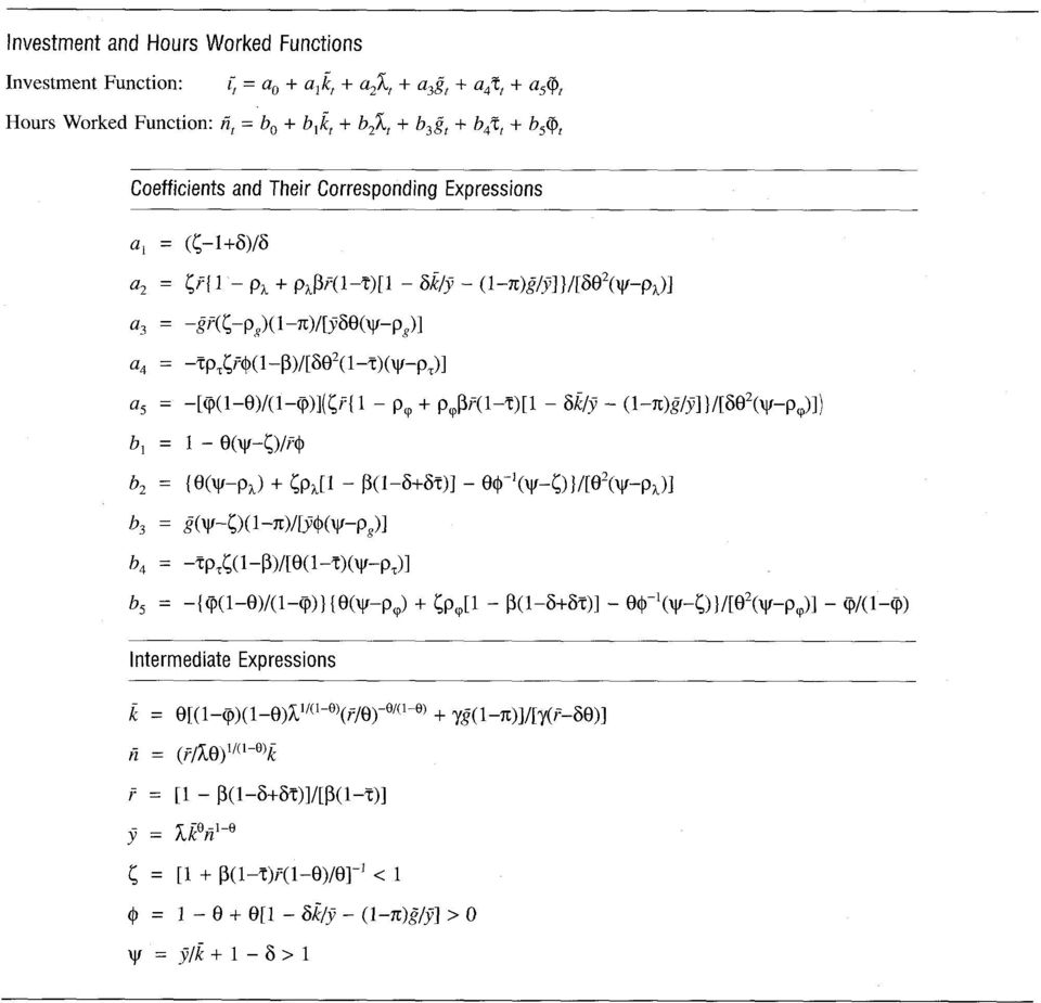
7 constant vector in equation (17), [ ν =( λ,ḡ, τ, ϕ) ], is chosen so that λ =1,ḡ/ȳ= 0.225, τ = 0.5, and ϕ = For the elements of the covariance matrix, Σ, I use variances and covariances from the data. (Again, I match correlations of the model series with those in the data after logging and detrending both, using the method of detrending from Prescott 1986.) The parameter estimates appear in the footnote of Table 2. The results from simulating the model with variable tax rates and government consumption are presented in Table 2. Compare the first column of statistics for U.S. data with the second column of statistics for the divisible-labor model with utility function defined by (17). Recall that the main failures of the standard model are its inability to generate the observed variability in consumption, hours worked, and productivity and its inability to generate a near-zero correlation between hours worked and productivity. With fiscal shocks included, the model is in much better agreement with the data; consumption, hours worked, and productivity are more variable. The standard deviation for consumption is 0.98 percent, which is close to that observed in the data (0.91). The standard deviation of hours worked is 1.31, which is significantly higher than that predicted by the standard model (0.89). Even if I take into account the standard deviations of the simulated series, I find a significant improvement. The third column of Table 2 has statistics for the indivisible-labor model with utility defined by (19). Note that a larger elasticity of labor supply and variable labor tax rates imply that the standard deviation of hours worked is 2.03, which is significantly higher than that of the data. Similarly, the output and investment are too variable in this case. In Table 3, I report statistics for the model with constant tax rates and government consumption. In this case, I set ρ ν = 0 and Σ = 0. An earlier comparison of statistics for the United States and the standard model (in Table 1) revealed that the variability of consumption, hours worked, and productivity is too low in the standard model. But the variability of hours worked is even lower if the fiscal variables (tax rates and government consumption) are set equal to their sample means, because the response of investment and labor to technology shocks depends on the level of the fiscal variables. For example, the higher the tax rate on labor, the smaller the incentive to increase hours worked in response to a positive technology shock. If I hold the fiscal variables constant in the indivisiblelabor model, I get a similar result. The higher the fiscal variables, the smaller the response of output, investment, and hours worked to technology shocks. These results suggest that adding constant fiscal variables will generate worse agreement with U.S. data than the standard model. In summary, what I find is that the model with divisible labor [that is, utility defined by (17)] and variable tax rates and government consumption does a better job than the standard model or Hansen s (1985) indivisible-labor model in accounting for fluctuations in output and employment. Furthermore, by adding constant tax rates and government consumption to the standard model, I show that the contribution of technology shocks to fluctuations in output and employment is significantly less than predicted by Kydland and Prescott (1982). Conclusion The two extensions of the standard Kydland-Prescott (1982) business cycle model explored here make different assumptions. And their results vary in how much they move business cycle research toward the goal of producing a model that reliably mimics the cyclical patterns in U.S. data. In the first extension, Hansen (1985) assumes that some fraction of the population works and some fraction does not. The result is that although his model captures the response of labor to technology shocks, it fails to capture the observed variability in consumption and the near-zero correlation between hours worked and productivity. In the second extension, I assume that agents substitute between taxable and nontaxable activities in response to fiscal shocks. The result is a model that can account for most of the observed variability in consumption and hours worked. Adding fiscal shocks to the standard Kydland- Prescott model significantly improves its ability to mimic the fluctuations of U.S. aggregate data. *The author thanks Rao Aiyagari, Toni Braun, Bob King, Kathy Mack, Art Rolnick, Dave Runkle, Martie Starr, and Chuck Whiteman for comments on earlier drafts. 1 In McGrattan 1994a, I explicitly account for growth in the time series of the model and data. Here, I am implicitly assuming that the model time series are fluctuations around some growth trend. Therefore, I assume 1 < ρ λ <1. 2 See McGrattan 1994a and 1994b for more details on the numerical methods for computing equilibria in the models of this article. 3 In McGrattan 1994a, I describe how to compute maximum likelihood estimates for a similar model. In that case, all first and second moments of the data are used when identifying the parameters. I also show that the contribution of technology shocks to fluctuations in output is close to 40 percent for U.S. data, which is significantly smaller than Prescott s (1986) estimate of 75 percent. 4 As in footnote 1, I assume that the eigenvalues of ρ ν are inside the unit circle. 5 A similar set of equations can be derived for the specification of (17). They are more complicated and yield similar results to those derived here. Appendix A Labor and Investment Decision Functions This appendix describes the optimal investment and labor decision functions for one of the model economies in the preceding paper. [See the section in the preceding paper on the model with fiscal shocks and the utility function given in (19).] This economy has four sources of fluctuations. Technology shocks, which are the sole source of fluctuations in the standard model, are one source. Government consumption and two tax rates one on capital and the other on labor are the other three sources of fluctuations in this economy. The accompanying table displays the investment and labor decision functions for this model economy. To simplify the analysis, I assume that ρ ν of (23) in the preceding paper is diagonal with diagonal elements equal to ρ λ, ρ g, ρ τ, and ρ ϕ. Note that the approximate decision functions for investment and labor are linear. The tilde ( ) over the variable implies that it is normalized by its mean; that is, k t = k t / k. 1 The normalization of the state and decision variables by their mean allows for a simple interpretation of the coefficients. The coefficients measure the percentage change in investment or labor in response to a one percent change in one of the state variables. For example, if the government consumption is one percent above its average level and the capital stock, k, the technology shock, λ, the capital tax rate, τ, and the labor tax rate, ϕ, are equal to their average levels, that is, k t = k, λ t = λ, τ t = τ, and ϕ t = ϕ, then hours worked will have increased by b 5 percent. The coefficients in the investment and labor decision rules of the table are functions of the underlying parameters of preferences (β,γ,π), technology (θ,δ, λ,ρ λ ), and government policy (ḡ, τ, ϕ,ρ g,ρ τ,ρ ϕ ). From these parameters, I can construct the average rate of return on capital, r, the average level of the

8 capital stock, k, the average hours worked, n,and the average level of output, ȳ. To simplify the formulas, I also include intermediate parameters φ, ψ, and ζ. Households response to a technology shock, the first source of fluctuations in the model, changes when other shocks are included. That is, the signs and relative magnitudes of the coefficients affect the estimates of the contribution of the technology shock and of fiscal variables to aggregate fluctuations. For example, the magnitudes of the coefficients on the technology shock, λ, are quite different for the models with and without fiscal shocks. If I use the parameterization of Table 1 from the preceding paper, then a 2 = 5.16 and b 2 = But if I use the parameterization of Table 2 from the preceding paper, then a 2 = 4.00 and b 2 = Thus, if tax rates and government consumption are included, the model predicts a much smaller increase in investment and hours worked to an increase in the technology shock. In effect, households are less willing to increase investment and hours worked when these activities are being taxed. A second source of fluctuations is variation in government consumption. The coefficients a 3 and b 3 in the accompanying table can be used to determine the effects of a change in government consumption. A one percent change in government consumption, with all other state variables fixed, leads to an a 3 percent increase in investment and a b 3 percent increase in hours worked. Suppose, for example, that π is strictly less than one. In this case, whether the response of investment to an increase in government consumption is positive or negative depends on the sign of ζ ρ g. If I use the parameterization of Table 2 from the preceding paper, ζ = 0.963, which is not much different from ρ g = Thus the response of investment to an increase in government consumption is small but positive. The response of hours worked to an increase in government consumption is also positive. If I use the parameterization of Table 2 from the preceding paper, I find b 3 = Thus a one percent increase in government consumption leads to a little more than a onefourth percent increase in hours worked. Note that if increases in government consumption were temporary (so ρ g = 0), then the model would predict a smaller response in hours worked and less variation in hours over the cycle. If π = 1, households do not adjust investment and hours worked in response to shocks to government consumption. This result can be easily explained by considering the household s utility function. If π = 1, then what matters to the household is the sum of private and public consumption. Thus households respond to increases in g t with offsetting decreases in c t while leaving investment and hours worked unaffected. The more variation in g t, the more variation in c t. In this case, government consumption affects investment and labor only indirectly. The average level of consumption, ḡ, affects the responses of these decision variables to other shocks. A third source of fluctuations is variation in the tax rate on capital. The coefficients on the tax rate in the investment and labor decision functions are given by a 4 and b 4 in the accompanying table. These formulas imply that investment and hours worked decrease in response to an increase in the tax rate on capital. As in the case of government consumption, the effects of the capital tax rate depend on how persistent the changes are. If changes in the tax rate are temporary (so ρ τ = 0), as Judd (1992) has argued, then the coefficients on the tax rate in both the investment and labor equations are zero. In that case, the tax on capital can significantly affect fluctuations only if the average level, τ, has a big effect on the other coefficients in the decision functions. Suppose, instead, that changes in tax rates are not temporary (so ρ τ > 0). If I use the parameterization of Table 2 from the preceding paper, then a 4 = and b 4 = As expected, tax rates on capital have a negative effect on both investment and hours worked. If the tax rate were 10.0 percent above its average value (that is, at 0.55 rather than 0.50), then investment would be 8.8 percent below average and hours worked would be 2.2 percent below average. The effect of changing capital tax rates also depends crucially on the discount factor, β, which is a difficult parameter to estimate. If households are very patient and thus put close to equal weight on present and future consumption (so β is close to 1), then they respond very little to changes in the tax on capital. That is, they do not adjust their saving behavior in response to shocks in tax rates on capital. A fourth source of fluctuations in the model economy is variation in the tax rate on labor. Shocks to the labor tax rate cause fluctuations in investment and labor if the coefficients a 5 and b 5 in the investment and labor decision functions are nonzero. If I use the parameterization of Table 2 from the preceding paper, then these coefficients are a 5 = and b 5 = Thus a 10.0 percent increase in the labor tax rate has a similar effect on investment as a 10.0 percent increase in the capital tax rate. The response of hours worked, however, is much larger for an increase in the labor tax rate than an increase in the capital tax rate. One interesting feature of this model is that the formulas for the coefficients on the labor tax rate (a 5,b 5 ) are very similar to the coefficients on the technology shock (a 2,b 2 ) when ρ λ = ρ ϕ. Therefore, if technology shocks have a large impact on investment and hours worked, then labor tax rates must also have a large impact on these decisions. Appendix B The Data Used in This Study The data used in the preceding paper are real aggregate data of the United States for the sample 1947:1 1987:4. All annual series (that is, capital and tax rates) are log-linearly interpolated to obtain quarterly observations. The final numbers were obtained by dividing the series listed by the population series given in the accompanying table. 1 I use the terms mean and average and the overbar symbol (-) to denote the steadystate value of variables for the nonstochastic version of the model. The steady states are solutions to the first-order conditions of the firm and household problems, if I assume that ε t = 0 for all t. References Barro, Robert J., and Sahasakul, Chaipat Average marginal tax rates from social security and the individual income tax. Journal of Business 59 (October, part 1): Braun, R. Anton Tax disturbances and real economic activity in the postwar United States. Journal of Monetary Economics 33 (June): Chang, Ly-June Business cycles with distorting taxes and disaggregated markets. Manuscript. Rutgers University. Hansen, Gary D Indivisible labor and the business cycle. Journal of Monetary Economics 16 (November): Hill, Martha S Patterns of time use. In Time, goods, and well-being, ed. F. Thomas Juster and Frank P. Stafford, pp Ann Arbor: University of Michigan Press. Internal Revenue Service (IRS). Various years. All returns: Sources of income (taxable income). In Statistics of income, individual income tax returns. Washington, D.C.: U.S. Government Printing Office. Joines, Douglas H Estimates of effective marginal tax rates on factor incomes. Journal of Business 54 (April): Judd, Kenneth L Optimal taxation in dynamic stochastic economies: Theory and evidence. Manuscript. Stanford University. Kydland, Finn E., and Prescott, Edward C Time to build and aggregate fluctuations. Econometrica 50 (November): McGrattan, Ellen R. 1994a. The macroeconomic effects of distortionary taxation. Journal of Monetary Economics 33 (June): b. A note on computing competitive equilibria in linear models. Journal of Economic Dynamics and Control 18 (January): Musgrave, John C Fixed reproducible tangible wealth in the United States: Revised estimates. Survey of Current Business 66 (January):

9 Fixed reproducible tangible wealth in the United States, Survey of Current Business 67 (August): Prescott, Edward C Theory ahead of business cycle measurement. Federal Reserve Bank of Minneapolis Quarterly Review 10 (Fall): Also, 1986 in Real business cycles, real exchange rates and actual policies, ed. Karl Brunner and Allan H. Meltzer. Carnegie-Rochester Conference Series on Public Policy 25 (Autumn): Amsterdam: North-Holland. Rogerson, Richard Indivisible labor, lotteries and equilibrium. Journal of Monetary Economics 21 (January): Seater, John J On the construction of marginal federal personal and social security tax rates in the U.S. Journal of Monetary Economics 15 (January): Summary fixed reproducible tangible wealth series, Survey of Current Business 68 (October): U.S. Department of Commerce. Various years. Bureau of Economic Analysis. Table 1.2. In The national income and product accounts of the United States, statistical tables. Washington, D.C.: U.S. Government Printing Office. U.S. Department of Health and Human Services. Various years. Social Security Administration. Tables 2 and 4. In Social security bulletin. Washington, D.C.: U.S. Government Printing Office. U.S. Department of Labor. Various years. Bureau of Labor Statistics. The employment situation. Washington, D.C.: U.S. Government Printing Office.

10

11

12

13

14

15