Data Based on Fisherman's Self-Confessment

Transcription

1 M e a s u r i n g V a l u e - A d d e d i n H i g h e r E d u c a t i o n Jesse M. Cunha Assistant Professor of Economics Naval Postgraduate School jcunha@nps.edu Trey Miller Associate Economist RAND Corporation tmilller@rand.org September 2012

2 We thank the Texas Higher Education Coordinating Board for its support of this project, particularly Susan Brown, David Gardner and Lee Holcombe. This paper has benefited from comments and suggestions from participants in the Bill & Melinda Gates Foundation / HCM Strategists Context for Success Project. Doug Bernheim, Eric Bettinger, David Figlio, Rick Hanushek, Caroline Hoxby, Giacomo De Giorgi and Paco Martorell provided helpful comments and suggestions at various stages. This work updates and extends a 2008 report we wrote for the Texas Higher Education Coordinating Board entitled Quantitative Measures of Achievement Gains and Value-Added in Higher Education: Possibilities and Limitations in the State of Texas. Student achievement, which is inextricably connected to institutional success, must be measured by institutions on a value-added basis that takes into account students academic baseline when assessing their results. This information should be made available to students, and reported publicly in aggregate form to provide consumers and policymakers an accessible, understandable way to measure the relative effectiveness of different colleges and universities. I n t r o d u c t i o n Quote from A Test of Leadership, the 2006 Report of the Spellings Commission on Higher Education As exemplified in this quote from the Spellings Commission report, an outcomes-based culture is rapidly developing amongst policymakers in the higher education sector. 1 This culture recognizes (i) the need for measures of value-added, as opposed to raw outcomes, in order to capture the causal influence of institutions on their students, and (ii) the power that value-added measures can have in incentivizing better performance. While many U.S. states currently have or are developing quantitative measures of institutional performance, there is little research for policymakers to draw on in constructing these measures. 2,3 In this paper, we outline a practical guide for policymakers interested in developing institutional performance measures for the higher education sector. As our proposed measures adjust, at least partially, for pre-existing differences across students, we refer to them as input-adjusted outcome measures (IAOMs). We develop a general methodology for constructing IAOMs using student-level administrative data, we estimate IAOMs for one large U.S. state, and we discuss the merits and limitations of the available data sources in the context of our empirical analysis. 4 The rapid transition toward an outcomes-based culture in the higher education sector mirrors recent trends in the K-12 sector. Research in K-12 schools has shown that accountability-based policies can indeed increase performance in these settings. 5 While assessment and accountability are no less important in higher 2

3 education, two differences render impractical the wholesale importation of the K-12 model to higher education. First, year-on-year standardized test scores are unavailable in higher education. Test scores are a succinct and practical way to assess knowledge; compared year-to-year, they provide an excellent measure of knowledge gains. Furthermore, year-to-year comparisons of individuals allow a researcher to isolate the influence of specific factors, such as teachers and schools, in the education process. Without standardized tests, we are forced to rely on other outcomes in higher education, such as persistence, graduation and labor market performance. Second, students deliberately and systematically select into colleges. 6 Combined with the lack of year-onyear outcome measures, this selection problem can plague any attempt to attribute student outcomes to the effect of the college attended separately from the effect of pre-existing characteristics such as motivation and natural ability. The methodology we propose to address these issues involves regressing student-level outcomes (such as persistence, graduation or wages) on indicators of which college a student chooses to attend, while controlling for all observable factors that are likely to influence a student s choice of college (such as demographics, high school test scores and geographic location). This exercise yields average differences in measured outcomes across colleges, adjusted for many of the pre-existing differences in the student population that is, IAOMs. Given the degrees of freedom typically afforded by administrative databases, we recommend that researchers include as many predetermined covariates that are plausibly correlated with the outcome of interest as possible. This approach allows one to minimize the extent of omitted variable bias present in IAOMs, but it is unlikely to capture all factors that influence a student s choice of college. To the extent that these unobserved factors drive the observed cross-college differences in outcomes, the resulting IAOMs cannot be interpreted as causal. We discuss the implication of this fundamental concern in light of practical policymaking in higher education. Furthermore, we provide a description of types of data that may be available in higher education databases in general, recognizing that the data are a limiting factor for the number and quality of IAOMs that policymakers can develop. These data include administrative records from higher education agencies, agencies overseeing public K-12 schools and agencies responsible for administering unemployment insurance benefits. Policymakers may also purchase data from external providers, such as SAT records from the College Board. 3

4 Fundamentally, the choice of data to be collected, and the resulting quality of IAOMs that can be developed, is a policy choice. While collecting more data increases the quality of IAOMs, it also increases the cost of data collection and processing. Thus, collecting additional data for the sake of IAOMs alone is inadvisable unless it is expected to sufficiently improve the quality of metrics. We implement our methodology using rich administrative records from the state of Texas, developing IAOMs for the approximately 30 four-year public colleges. Texas has one of the most-developed K-20 data systems in the nation; as such, it is an ideal setting to demonstrate the incremental benefits of collecting and using various student-level data sources to input adjust, while at the same time demonstrating the potential bias we face by not using certain data. This information is certainly useful for policymakers who have access to K- 20 data systems that are less developed than those in Texas. Not surprisingly, the results confirm that IAOMs change considerably as more controls are added. Not controlling for any student characteristics, we find large mean differences in outcomes across public colleges. For example, the mean difference in earnings between Texas A&M University and Texas Southern University the institutions with the highest and lowest unconditional earnings, respectively is 78 percentage points. Upon controlling for all of the data we have at our disposal, the difference in mean earnings between Texas A&M and Texas Southern decreases to 30 percentage points. A similar pattern is seen when using persistence and graduation as outcomes, and when comparing amongst various student subgroups. Furthermore, we find large variance in IAOMs over time. We conclude by enumerating specific recommendations for practitioners planning to construct and implement IAOMs, covering such issues as choosing empirical samples, the cost of data collection, the choice of outcomes, and the interpretation of IAOMs from both a statistical and policy perspective. 2. Q u a n t i f y i n g t h e i m p a c t o f h i g h e r e d u c a t i o n Colleges aim to produce a wide range of benefits. First, and perhaps foremost, is the goal of increasing general and specific knowledge, which increases students economic productivity. In general, higher productivity is rewarded in the labor market with a higher wage rate, which allows individuals more freedom to allocate their time in a manner that increases utility. 4

5 Second, knowledge may be valued in and of itself. This consumption value of knowledge certainly varies across students and, along with a host of other reasons, partially explains why students choose to select into non-lucrative fields. Third, higher education is generally believed to produce positive externalities. The most widely cited positive externality stems from productive workers creating economic gains greater than their own personal compensation. Another positive externality is social in nature, wherein informed, knowledgeable citizens can improve the functioning of civic society. 7 This discussion underscores the notion that institutional performance is inherently multi-dimensional. Quite likely, schools will vary in their performance across various dimensions, doing relatively well in one area but perhaps not in another. For example, a college may provide an excellent liberal arts education, imparting high levels of general knowledge about our human condition, but leave students with little ability to be economically productive without on-the-job training or further refinement of specific skills. We argue that quantitative measures of institutional performance at the postsecondary level necessarily require a set of indicators, as a single measure is unlikely to accurately aggregate these varying dimensions of performance. A full assessment of institutional performance thus requires a broad appraisal of indicators across an array of dimensions. However, the extent of the assessment is necessarily limited by the availability of data. 3. I d e n t i f i c a t i o n The fundamental empirical challenge we face is identifying the independent causal effect that a particular college has on an outcome of interest; however, it is well known amongst social science researchers that isolating such causal effects is not a trivial task. In this section, we first discuss the general statistical issues involved in causal identification and then discuss several specific empirical methodologies that policy analysts have at their disposal. 3.1 The identification challenge The identification challenge arises because we do not know what would have happened to a student if she had attended a different college from the one she actually did attend. Let us consider a student who enrolled at Angelo State University, a small college in rural Texas, and imagine we measure her earnings at some time in the future. The information we would like to possess is what her earnings would have been had she instead attended another college, such as the University of Texas (UT) at Austin, a state flagship research 5

6 university. If her earnings would have been higher had she attended UT Austin, we could conclude that, for this student, Angelo State performed worse along the earnings dimension than did UT Austin. Obviously, we could never know what our student s earnings would have been had she attended UT Austin or any other school, for that matter. These unobserved outcomes that we desire are referred to as missing counterfactuals, and the goal of our empirical research is to construct proxies for them. A fundamentally important issue involves understanding how closely the proxies we use reflect these missing counterfactuals. Given that we cannot clone students and send them to various colleges at once, a second-best way to overcome this identification problem is to imagine what would happen if we randomized students into colleges. The randomization would ensure that, on average, the mix of students with various pre-existing characteristics (such as ability, motivation, parental support, etc.) would be the same across different colleges. If the pre-existing characteristics of students are balanced across colleges, then the effects of these characteristics on outcomes should be balanced as well. Thus, we could conclude that any observed differences in average outcomes must be due to the effect of the individual college attended. Obviously, we have not randomly assigned students to colleges, and cannot do so; nonetheless, this is a useful benchmark with which to compare the available statistical methods discussed next. 3.2 Differences in means A simple, yet naïve, way to overcome the missing-counterfactual problem is to use the outcomes of students who attend different colleges as counterfactuals for one another. For example, we could compare the average earnings of all Angelo State students with the average earnings of students in the same enrollment cohort who attended UT Austin. While appealing, this solution will not recover the differential causal effect of attending Angelo State versus UT Austin if the students who enrolled at UT Austin are different from our Angelo State student along dimensions that influence earnings. For example, imagine that our Angelo State student had lower academic ability than the average UT Austin student. Furthermore, assume that high academic ability leads to higher earnings, regardless of which school one attends. The earnings of our Angelo State student and her counterparts at UT Austin are thus determined by at least two factors: (i) pre-existing differences in academic ability, and (ii) the knowledge gained while at the school they chose to attend. If we simply compare the earnings of our Angelo State student with those of her counterparts at UT Austin, we have no way of knowing whether the differences in their earnings are due to the pre-existing differences in academic ability or to the specific knowledge gained in college. 6

7 This differences-in-means approach can be implemented using a linear regression, where an outcome, Y i, that varies at the student level is regressed on a set of indicators, {E 1, E 2,,E n}, for enrollment in colleges {1,2,,n}: Y i 0 1 E 1i 2 E 2i... n E ni i 0, the constant, in this regression is the average outcome for students who enrolled at the school with the omitted indicator, and { 1, 2,, n} are the average outcomes for students who enrolled at schools {1,2,,n}. The error term, i, captures the deviation of individual outcomes from the mean outcome of the college that the student attended. We can think of all of the other variables that determine the outcome as being included in the error term. The selection problem can now be made precise using the language of regressions. If the omitted variables in i are correlated with both {E 1, E 2,,E n} and Y i, then estimates of { 1, 2,, n} will include not only the differential effect of attending each college but also all of the pre-existing differences included in i that determine Y i. That is, { 1, 2,, n} will be biased estimators of the independent causal effects of a college on the outcome in question. 3.3 Controlling for omitted variables The standard way to solve this omitted variable bias problem is to include as regressors the omitted factors that we believe are correlated with selection into college. For example, if we believe that higher-ability students will select into higher-quality colleges, and that higher-ability students would have earned higher wages regardless of which college they attended, then controlling for a measure of ability in the regression will help to remove the influence of ability. The regression model would thus be modified as follows, where X i is a vector of conditioning variables and is a vector of coefficients: Y i 0 1 E 1i 2 E 2i... n E ni X i i One can imagine controlling for all omitted variables in this way, thus completely solving the omitted variable bias problem. However, we are limited by the fact that we do not observe all omitted variables. For example, while we may be able to control for ability using scores on a standardized test, we are unlikely to find a quantifiable measure of motivation. The empirical exercise we advocate is thus one of controlling for as many omitted variables as possible. Using this approach, however, poses a fundamental problem in that we will never know whether we have fully controlled for all omitted variables that are correlated with college enrollment and the outcome of interest, and thus we can never know whether our regression coefficients are identifying a true causal effect 7

8 of the college on the outcome of interest. Thus, the degree to which the indicators defined by { 1, 2,, n} capture causal differences across colleges is determined by the extent of omitted variable bias eliminated by the control variables Choice of control variables Which covariates, then, should we include in our model? Given the sample sizes that are typically included in administrative databases, the goal should be to include as many pre-determined student or high school level covariates as possible that could plausibly affect the outcome of interest. The fundamental limitation in this endeavor is the types of data that are included in, or can be merged to, state administrative data systems. Data typically available include college enrollment records; student records from high school, including scores on state-administered tests; SAT and/or ACT records from the College Board; and, in some cases, college application records. We discuss these data and procedures for merging them in more detail below. A general rule, however, is that one should include only covariates that are predetermined at the time of college entry; that is, covariates should not be affected by the student s choice of college. 8 Otherwise, estimates of { 1, 2,, n} would exclude the indirect effect of these variables on the outcome of interest. A particularly salient example of this principle is whether to include college major as a covariate, as for some students the choice of major will be affected by the college they choose to attend. For example, consider a student who wants to attend the College of Engineering at UT Austin but is only admitted to the College of Liberal Arts at UT Austin and the College of Engineering at the University of Houston. This student might choose to attend UT Austin, and his choice of college major would be determined by his college choice. If college major affects our outcome of interest, then we would want to include the indirect effect of college major in our performance indicator. Thus, variables such as college major that are not predetermined, and hence could be affected by college choice, should rightfully be considered as outcomes rather than covariates Applications as control variables One set of conditioning variables deserves particular discussion: the set of schools to which a student applied and was accepted. Dale and Krueger argue that conditioning on this profile of applications and acceptances captures information about the selection process that would otherwise be unobserved by the researcher. 9 Specifically, they argue that students use private information to optimize their college application decisions, and colleges use information unobservable to researchers (such as the quality of written statements and letters of recommendation) to make acceptance decisions. Thus, students with 8

9 identical college application and acceptance profiles are likely to be similar on both observable and unobservable dimensions. In essence, this methodology identifies the performance of, say, UT Austin relative to, say, Texas A&M University (TAMU) by restricting attention to students who applied to both UT Austin and TAMU (and possibly other colleges), and comparing the outcomes of those who subsequently enrolled at UT Austin to the outcomes of those who enrolled at TAMU. Of course, it is unreasonable to assume that this conditioning exercise controls perfectly for selection into college. In particular, the identification strategy boils down to comparing students with the same observable characteristics who applied to and were accepted at the same set of colleges yet decided to attend different colleges. It would be naïve to believe that this ultimate choice of which school to attend was random. For example, if a student was accepted at both UT Austin and Angelo State University, why would he choose to attend Angelo State? Perhaps he received a scholarship to Angelo State, or maybe he wanted to live with family in San Angelo. These are omitted variables that may also impact outcomes. Thus, the concern is that if the final choice of which college to attend is nonrandom, then there may be remaining omitted variable bias. Despite these caveats, conditioning on observable student characteristics such as SAT scores and high school GPA is likely to remove much of the first-order bias arising from sorting on ability. Nevertheless, we do not claim that any of the models we use deliver IAOMs that are completely free of omitted variable bias. 3.4 Other methods for recovering causal effects Despite the caveats inherent in the conditioning-on-observables regression methodology outlined above, we believe that this empirical exercise can be extremely useful for policymakers. Furthermore, without randomized controlled trials or natural experiments, which are often narrow in scope, this conditioning methodology may offer the best evidence available. Nevertheless, several other methods are worth discussing. Natural experiments One method exploits variation in enrollment patterns that are plausibly exogenously determined, allowing the researcher to mimic the randomization process and estimate the causal impact of attending particular colleges.10,11 For example, Hoekstra exploits a strict SAT score cutoff used for admission by a large flagship university to compare the earnings of applicants scoring just above and below the admission cutoff and finds that those students just admitted had a 20 percent earnings premium eight years after admission. Unfortunately, these methods are in general available only in narrow contexts. 9

10 Fixed effects Another method uses changes in an outcome before and after receiving education in order to net out bias stemming from missing variables that are constant over time. This fixed effects methodology requires observing an outcome more than once. While it is favored in the K-12 sector when test-based outcomes are observed on an annual basis, it is unlikely to be of use in the postsecondary sector as most available outcomes, such as graduation rates or earnings, are not observed before entering college. 12,13 4. Data, sample and variable construction Governments face an important policy question in choosing what data to collect on the students in their higher education system, whether to collect unique student identifiers that allow researchers to track individuals into other databases, and what other databases to include in their education data systems.14 Viewed from the standpoint of producing meaningful input-adjusted output measures, the more data states collect on students, the better. However, collecting data is costly in terms of compliance costs, direct monetary outlays and potential disclosure risk. 15 One issue with state data systems and other mergeable student-level data is that they are typically collected for specific purposes unrelated to constructing IAOMs. For example, UI records are designed to determine eligibility and benefit levels for state-administered Unemployment Insurance programs, and hence include information on quarterly earnings for benefits-eligible jobs rather than wages for all jobs. This means that many of the data included in state data systems require considerable manipulation for researchers to produce useful input-adjusted output measures. Researchers and policymakers must therefore be careful in interpreting measures generated from these data. In this section, we first describe the types of student-level data that can be used to measure achievement gains in higher education. We then discuss issues surrounding the availability and collection of these data, emphasizing the costs of collection versus the benefits of individual data sources, the construction of outcome indicators, and missing data. We conclude with a description of the data sources available in the state of Texas, which are used in the empirical analysis below. 4.1 State higher education data systems Many states collect individual-level data on students attending the institutions in their higher education systems. These databases are primarily used by state education agencies to calculate institutional funding, 10

11 and this is reflected in the types and formatting of data they collect. Many states also use state higher education data to conduct internal research and respond to data requests from government officials. Since most states fund institutions on a semester credit hour basis, state higher education databases typically have detailed individual-level information on semester credit hours attempted and/or completed at each institution attended, often broken down by area or level of instruction. States that collect this information typically also collect basic demographic information about their students, including race, ethnicity and gender. States must also compute college graduation rates for research and/or funding purposes, so most states collect individual-level data on college degrees earned. Some states collect more refined information on students attending their higher education systems including but not limited to college major, GPA, individual course enrollment and grades in individual courses. Texas also collects detailed information on college applications. Data in state higher education data systems can be used to create both key outcomes and important predetermined control variables for use in input-adjusted output measures. Outcomes include primary indicators such as persistence and graduation, as well as secondary indicators such as performance in developmental courses, transition rates to other campuses and enrollment in graduate school. Predetermined control variables that may be available in state databases include demographic indicators and, where collected, information on college application records. 4.2 Other data sources that can be merged with higher education data K-12 data In order to comply with the NCLB Act, states have developed extensive databases at the K-12 level that include student-level scores on standardized tests, demographics (such as race, ethnicity and gender), and free lunch status (an indicator of family income). Many states collect even more information, such as high school GPA and high school courses taken. If these data contain unique student identifiers (such as SSNs or name and date of birth), they can be merged with college-level databases. These data are useful as control variables that help reduce omitted variable bias, as the information is determined prior to the college enrollment decision. Administrative earnings records Quarterly earnings data are often collected by state agencies in charge of administering the state s Unemployment Insurance (UI) benefits program In most cases, UI earnings records can be merged with higher education data systems via student SSNs. 11

12 SAT and ACT data States can purchase SAT and ACT test score data when the state higher education data system contains unique identifying information such as SSNs or student names and dates of birth. In addition to test scores, these databases include indicators for the set of institutions to which students sent their test scores and several survey questions collected at the time of testing. The surveys have useful predetermined control variables, including self-reported GPA, class rank, planned education attainment, and father s and mother s education level. 4.3 Constructing a base sample and merging data Researchers face a number of choices in constructing data files for analysis, and these choices can have major implications for the resulting input-adjusted output measures. Researchers must choose a base sample of students on which to base input-adjusted output measures and decide how to treat missing data. Researcher choices reflected in the construction of outcome variables are more likely to affect resulting IAOMs than those reflected in the construction of control variables Constructing a base sample Researchers must choose the base sample of students to track through college and possibly into the labor market. Should researchers focus on all entering college freshmen, all in-state students, all students who took the ACT and/or SAT, or all graduates of the state public K-12 system? As we demonstrate below, IAOMs are highly sensitive to these choices. We recommend that researchers implementing IAOMs consult with policymakers in order to define a sample that best reflects the state s policy goals. In some cases, policymakers may care differentially about student subgroups. For example, policymakers may care about the outcomes of in-state students more than those of out-of-state students. In such cases, researchers should consider developing multiple measures based on each subgroup, so that policymakers can develop a proper assessment of institutional success Merging databases Once researchers have chosen a base sample, they must merge data over time and across databases in order to develop outcome variables and predetermined control variables to include in the analysis. This process introduces missing data for three key reasons. First, it may be impossible to track students across databases in some cases. For example, if the unique identifier included in the higher education data system is based on SSNs, then it is impossible to merge high school graduates without SSNs into other databases. In this case, researchers cannot include these students in the base sample. 12

13 Second, it is often the case that students in one database will not be included in another. For example, a student who enrolled at UT Austin might have taken the ACT, and hence does not show up in the SAT data. Finally, students may have missing data for some variables within a database. For example, many students do not complete the entire SAT or ACT survey. In these two cases, researchers can drop students with missing data for any variable, but this can lead to sample selection bias, so we do not recommend doing so. Instead, we recommend that researchers create dummy variables indicating that the variable is missing and include those observations in the model. This procedure maximizes the identification that the variable affords without introducing sample selection bias, and is common in the economics literature in cases where there are many variables with missing data for some observations Constructing variables Researchers face many choices in constructing variables for analysis. For example, how do we control for race/ethnicity when there are 10 different categories for those variables? How do we code institution of enrollment when students may attend more than one institution in a given semester? Do we code persistence as remaining enrolled in a particular institution or any institution? These choices can have major impacts on the resulting input-adjusted output measures. Researcher choices that affect the construction of specific control variables (e.g., how SAT scores are entered in the model) are unlikely to affect resulting input-adjusted output measures, particularly when many control variables are included in the model. The notable exception to this rule is when policymakers are concerned with outcomes for a particular subgroup so that subgroup-specific measures should be developed. For example, if policymakers are interested in input-adjusted graduation rates for minority students, whether a researcher classifies Asians as minorities may be important. In such cases, we recommend that researchers consult with policymakers to define control variables in the way that best reflects state priorities. Input-adjusted output measures have the potential to be considerably more sensitive to the construction of outcomes. In the remainder of this section, we discuss issues related to the construction of input-adjusted graduation and persistence rates, and earnings, and the use of these measures for policymaking Graduation and persistence rates Researchers face a number of decisions in constructing completion and persistence rates. Should researchers calculate rates based on retention within a single institution or in any institution? Should persistence be 13

14 based on semester credit hours attained or year-to-year attendance? Should researchers use four- or six-year completion rates? In general, we recommend that researchers communicate closely with policymakers to choose the construction method that best reflects state goals. While properly constructed input-adjusted graduation and persistence rates are potentially useful tools for policymakers, it is important to keep in mind the lag time required to calculate them. Most bachelor degrees have four-year degree plans, but many students take six years or more to complete them. Thus, inputadjusted output measures should exhibit a four- to six-year lag in response to policy changes. On the other hand, one-year persistence rates can potentially respond to policy changes in the year following implementation. In general, we recommend that policymakers communicate with institutions when basing incentives on measures with a long lag time Earnings UI records have two key limitations. First, they include earnings only from jobs that are eligible for UI benefits. These include the majority of earnings from wages and salaries but exclude other sources, such as self-employment income. UI records also exclude earnings from federal government jobs, including those in the military. UI earnings thus systematically underreport total earnings, but this is a concern for our methodology only if students who attend some institutions are more likely to generate earnings from uncovered sources than are students who attend other institutions. Another limitation is that since UI records are maintained by states, they contain earnings information only for jobs held within the state. This means that states can use UI records to track only the earnings of college students who maintain residence in the state. This is a concern if students attending one institution are more likely to move out-of-state than students attending others, or if, for example, students who are employed out-of-state have systematically higher or lower earnings than those employed in-state. The extent of these biases will vary by state according to the likelihood of students seeking employment out-of-state. Thus, in states such as Wyoming and Vermont, with high out-migration rates, these concerns would be greater than in a state such as Texas, where students are more likely to remain in-state. On the other hand, policymakers may be more concerned with the outcomes of students who stay in-state, so in this case it would make sense to condition the sample on whether students remain in-state. Finally, the literature suggests that earnings during and immediately following college are highly variable, as it takes time for students to find appropriate job matches in the labor market. Thus, to calculate useful inputadjusted earnings outcomes, researchers must allow students sufficient time not only to complete college but also to be fully absorbed by the labor market. We recommend that researchers measure earnings at least 14

15 eight years after initial college enrollment, and preferably longer. Unfortunately, this restriction implies that input-adjusted earnings measures will have at least an eight-year lag from policy implementation to measure response, rendering the utility of these measures as a policymaking tool questionable, at best. 4.4 Data currently available in the state of Texas A key focus of this report is to explore the sensitivity of input-adjusted output measures to the issues discussed above. Toward that end, we use data collected by the Texas Higher Education Coordinating Board. These data are ideally suited to the task at hand, as they contain all of the major components discussed above. In particular, the Texas data have: K-12 data system, containing extensive information on demographics and high school coursetaking for all graduates of Texas public high schools; higher education data system, containing extensive information on college enrollment, degree attainment, GPA and performance in developmental courses, and college application records for all students attending four-year public colleges in the state; College Board data, including SAT scores and student survey information for all public high school graduates who took the SAT; and UI records, quarterly earnings data for all workers employed in benefits-eligible jobs in the state. We use the Texas data to develop input-adjusted output measures of college completion and two-year persistence rates, and earnings. Our fully specified model includes demographics and high school coursetaking patterns from state K-12 data, SAT scores and survey information from the College Board, and college application and acceptance profiles from the state higher education database. Table 1 summarizes the data we use, and we discuss the variables in turn in the next section. 5. Empirical specifications and results As discussed above, the main specification is a simple linear regression model of an outcome of interest regressed on a set of college enrollment indicators and various sets of control variables. In all of the models presented, we exclude the indicator for enrollment at Texas A&M University so that the resulting IAOMs can be interpreted as the mean difference in the outcome between Texas A&M and the institution represented by the corresponding dummy variable Outcome: Earnings We begin by examining how the input-adjusted earnings change upon controlling for various sets of observable covariates. If we believe selection into colleges will bias estimates, then controlling for successively more determinants of the college selection process should deliver IAOMs that are closer to the true causal impacts of attending different colleges. 15

16 Table 2 uses the logarithm of earnings eight years after graduating from high school as an outcome. 19 Column 1 conditions only on high-school graduation year fixed effects, which absorb any aggregate differences in earnings across years, such as the effect of inflation or general macroeconomic shocks. Thus, the coefficients in Column 1 can be interpreted as the average differences in unconditional earnings of enrollees at various Texas colleges, relative to enrollees at Texas A&M. For example, UT Dallas enrollees earned on average 12 percentage points less than Texas A&M enrollees, while Texas Southern University enrollees earned on average 78 percentage points less than Texas A&M enrollees. The results in Column 1 serve as a base case that can be compared with models that use predetermined covariates to partially remove omitted variable bias. Perhaps not surprisingly, the relative differences in unadjusted log earnings presented in Column 1 correlate highly with common perceptions of college quality published in the popular press such as U.S. News & World Report or Barron s Magazine. Finally, note that all of the estimates in Column 1 are significantly different from zero at the 1 percent level; that is, we are fairly confident that average unconditional earnings of students who initially enroll at Texas A&M are significantly higher than those of students who initially enroll in any other four-year public institution in Texas. 20 Columns 2 through 5 add the following sets of control variables sequentially: (i) race and gender controls, (ii) high school fixed effects and indicators for courses taken during high school, (iii) SAT score and various student and family demographics collected by the College Board, and (iv) application group fixed effects. The order of addition roughly reflects additional costs to a state: Race and gender are likely available in any higher education database; high school information requires coordination with the state K-12 Education Agency and the ability to link higher education records to K-12 data; SAT information is costly to acquire and requires coordination with the College Board and the ability to link to external databases with individually identifiable information; and college application data are uncommon and costly to collect but are available in Texas. Our main interest is in how input-adjusted output measures change with the number and types of predetermined control variables included in the model. Comparing across the columns of Table 1, several observations are worth noting. First, the range of point estimates shrinks as more controls are added. For example, the absolute range is 78 percentage points in Column 1, 43 percentage points in Column 3 and 30 percentage points in Column 5. This trend is consistent with a story in which students select into colleges according to innate ability; for example, students with high innate ability are more likely to attend Texas A&M, while students with relatively lower innate ability are likely to attend Texas Southern University. 16

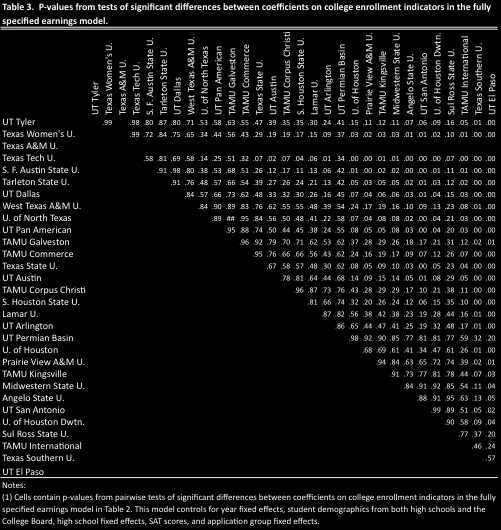
17 Therefore, controlling for these predetermined covariates that are correlated with ability reduces the disparity in earnings across institutions perceived to be of high or low quality, bringing the estimates closer to the true causal effects of colleges. Second, some sets of covariates change resulting IAOMs much more than others. For example, moving from Column 1 to Column 2 (controlling for race and gender in addition to year fixed effects) changes coefficients much less than moving from, say, Column 2 to Column 3 (additionally controlling for high school fixed effects and high school course taking indicators). 21 Regression theory informs us that these patterns reflect the degree to which the omitted variables are correlated with the included regressors and the outcome. Put differently, IAOMs will change depending on the information that is contained in the new control variables. 22 Third, the model with the most comprehensive set of covariates currently available in Texas stands out because many of the differences between Texas A&M and other universities become insignificant, as seen in Table 5. The loss of significance informs us that we cannot statistically distinguish the differential inputadjusted earnings across these schools. For example, while the point estimate for Texas State University is -.05, indicating that Texas State enrollees earn 5 percent less than Texas A&M enrollees on average, we cannot determine whether this difference is due to true differences in institutional performance or to chance. It is important to note that, while we do not believe that the model in Column 5 has fully solved the omitted variable bias problem, we do believe that further controlling for omitted variables will most likely reduce significant differences further. Thus, from a policy perspective, it would be unwise to conclude that Texas A&M performs better than Texas State along the earnings dimension. 5.2 Significant differences across colleges While informative, Table 2 shows directly the significance of earnings differences only between Texas A&M and all other institutions; it does not directly show us the difference in earnings between all other pair-wise combinations of institutions. From a policy point of view, this information is crucial, as it allows us to separate truth from noise in a meaningful way. One way to summarize this information is demonstrated in Table 3, which contains a matrix of p-values from pair-wise tests of significance of the coefficients in Column 5 of Table 2. The columns and rows in Table 3 are ordered as in Table 2, by order of the highest conditional earnings from the fully specified model. It is apparent that the point estimates are reasonably precise as we can detect significant differences between many colleges. 17

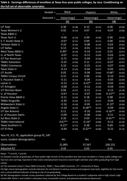
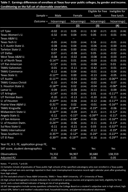
18 For example, the point estimate for Texas A&M is statistically larger than 14 of 30 Texas colleges. Interestingly, we cannot say with any degree of confidence that students attending UT Permian Basin, a small regional college located in West Texas, earn less on average than observationally equivalent students at Texas A&M. However, this is due to a large standard error that is partially a result of the relatively small number of students attending UT Permian Basin. 5.3 Outcomes: Persistence and graduation rates We now investigate one-year persistence rates and graduation rates as outcomes. In the interest of brevity, we display in Table 4 only results from the fully specified model that includes the largest set of covariates used in Column 5 of Table 1; however, qualitatively similar patterns as in Table 2 result from the successive addition of covariates with persistence and graduation as outcomes. Columns 1 and 3 of Table 4 include all college enrollees, while Columns 2 and 4 contain only enrollees with annual earnings greater than $2,000, the same sample as used in Table 2. Note that we order colleges in Table 4 as in Table 2, for ease of comparison. Focusing first on Columns 1 and 3, it is obvious that the ranking of schools is different from the ranking in the earnings regressions. For example, UT Tyler does relatively poorly in input-adjusted graduation rates (18 percentage points lower than Texas A&M), although it had the highest input-adjusted earnings in the state. In fact, Texas A&M has the highest input-adjusted graduation rate in the state (note that no coefficients are negative in Column 1). Turning to persistence rates in Column 3, there is once again a different ranking compared with both earnings and graduation. How should we view these results in light of the outcome measures on earnings in Table 2? In general, we believe that different outcomes capture different parts of the education production process and should lead to different IAOMs. Nevertheless, there is certainly correlation between persistence and graduation, in that you must persist to graduate, and we believe that more years of college must marginally lead to higher earnings, so persistence and graduation should correlate positively with earnings. However, the extent of this correlation is unknown and beyond the scope of this paper. Comparing Column 1 with Column 2, and Column 3 with Column 4, allows us to see how estimates change with the choice of sample. In general, we would expect the choice of sample to affect estimates, and this type of sensitivity should be examined by practitioners. If estimates do change, then we must be precise about what populations the samples represent. 18

19 In this example, both sample choices (all enrollees or only enrollees with earnings greater than $2,000) seem reasonable. There is no a priori reason why we would want to exclude enrollees with small or missing earnings, but if we are comparing estimates from persistence and graduation rate models to earnings models, it is useful to have the same sample. Table 4 shows that there is little movement in the point estimates across the samples. However, the general point remains that different samples will generally lead to different estimates. 5.4 Heterogeneous effects Stakeholders may be interested in the extent to which input-adjusted output measures vary across years. One way to examine this is to estimate our regression model separately by high-school graduation cohort, as in Table 6. A cursory look at a college s differential earnings with respect to Texas A&M shows there is significant movement. For example, UT Tyler enrollees vary from having the same conditional earnings as Texas A&M enrollees in 1998 to having 44 percentage points higher earnings in 1999 to having 24 percentage points lower earnings in As with all of our results, a more rigorous quantification of these changes must consider the statistical significance of the differences.23 However, given the sensitivity of IAOMs over time, we urge policymakers to use caution when interpreting IAOMs based on a single cohort of students, and we urge researchers to consider using multiple cohorts of students to construct IAOMs. Stakeholders may also be interested in the extent to which input-adjusted output measures vary by student subgroup. The same methodology used in Table 5 for comparing across years can be used in this case, and in Tables 6 and 7, we include input-adjusted earnings by race, gender and family income for the interested reader. 6. Conclusions and recommendations for constructing, interpreting and using input-adjusted output measures We conclude with a set of policy recommendations for practitioners interested in constructing and using input-adjusted output measures in higher education. In general, these measures can be a powerful tool for measuring the relative performance of higher education institutions. Properly constructed measures may also be useful to higher education institutions attempting to monitor their own performance and that of their peers, to students interested in attending college, and to employers interested in hiring college graduates. However, as our empirical results demonstrate, these measures are highly sensitive to seemingly trivial details related to their construction and will likely not represent the independent output of an institution. As such, improperly designed measures have as much potential to deceive stakeholders as inform them about true institutional quality, and we urge researchers to work with policymakers to construct measures in a way that best reflects their goals. 19

20 6.1 Recommendations concerning the choice of outcome measures 1) For a full assessment of institutional quality, develop a broad set of outcomes representing multiple dimensions of institutional performance. We have argued that institutional performance encompasses a broad range of dimensions that cannot be adequately captured in a single measure. A system of performance metrics allowing for an overall assessment of institutional quality is not unprecedented, and is consistent with the state of research and practice in the health sector. 24 2) Consult with policymakers and other stakeholders to choose a set of outcomes that (i) are of interest to the state and (ii) can be measured with quantitative data. While policymakers, students, university officials and other stakeholders are ideally suited to determine what needs to be measured, practitioners generally have better knowledge of what actually can be measured with the available data. Dialogue is necessary. 3) Consult with policymakers and other stakeholders to choose student subgroups that are of prime importance for each chosen outcome. Policymakers and other stakeholders may care differentially about the outcomes of different student subgroups such as in- versus out-of-state students, students with developmental needs, and/or students of various ethnic origins, and this may vary across outcomes. Researchers should work closely with key stakeholders to determine the student subgroups that are of most importance for each outcome measure. 4) Appraise the quality of indicators that can be developed with existing data, and identify priorities for additional data collection where needed. There is considerable variation across states in the types of data they collect on their students and in their ability to merge their databases to external sources. Researchers should appraise the data system in their state and assess the quality of indicators that they could develop with existing research. In doing so, they should identify priorities for additional data collection and, where possible, clearly delineate the benefits of the additional data. Researchers should work with policymakers to identify the costs of collecting the proposed additional data items. Costs may include in-house expenses of administrator time to purchase and/or collect and process additional data, as well as the excess compliance burden imposed on institutions and other state entities. 5) Work with policymakers to construct outcomes in a way that best reflects state goals. We have shown that seemingly trivial researcher choices about how to construct outcomes can have large impacts on resulting input-adjusted output measures. 6.2 Methodological recommendations for researchers 6) Once student subgroups defining the desired input-adjusted output measures have been set, create dummy variables as opposed to dropping observations with missing control variables. In merging 20

21 multiple databases across students and time, researchers are faced with how to treat missing data. The priority for input-adjusted output measures should be to reflect as closely as possible the causal impact of attending particular institutions for the relevant student subgroups. Once the subgroup has been set, we do not recommend dropping observations because of missing control variables. Instead, researchers should create dummy variables indicating the data for the corresponding observation that is missing. This procedure maximizes the identification that the control variables afford without introducing sample selection bias. 7) Include as many predetermined control variables that are potentially correlated with outcomes of interest as possible. Given the large sample sizes inherent with state databases, researchers should include these control variable to lessen potential omitted variable bias. 8) Do not include control variables that may be impacted by college choice. Input-adjusted output measures should come as close as possible to uncovering the causal impact of attending particular colleges on the chosen outcomes. If a variable may be affected by choosing a particular college, then its indirect impact should be included in the input-adjusted output measure. Where appropriate, variables that may be impacted by college choice can be considered as outcomes. 9) Use multiple cohorts of students to construct input-adjusted output measures. We have shown that input-adjusted output measures are highly variable over time. While some of this variance may be due to true year-to-year differences in institutional performance, much is likely due to noise. To minimize the impact of this instability, researchers should use multiple cohorts of students to construct input-adjusted output measures. 6.3 Recommendations related to the interpretation and use of input-adjusted output measures 10) Do not assume that input-adjusted output measures are causal. No matter how many predetermined control variables are included in a regression model, we can never be sure that estimates are unbiased. Moreover, we have shown that input-adjusted output measures are highly sensitive to variable construction and exclusion of various control variables. Policymakers and other stakeholders should bear this in mind when interpreting a set of input-adjusted output measures, and researchers should be careful to communicate the limitations of the measures that they produce. 11) Think in terms of broad classifications of institutional performance as opposed to specific rankings. We have shown that in Texas, adjusting outcomes for predetermined student characteristics makes it impossible to statistically distinguish outcomes across many sets of colleges. It would be unwise for public policy to distinguish between these statistically insignificant outcomes. In general, we urge policymakers to think in terms of broad classifications of institutional performance as opposed to 21

22 specific rankings. One possibility is to determine a benchmark and classify institutions as statistically below, within normal statistical variance of, or exceeding the specified benchmark. 12) Consider the potential for institutions to game the system. Experience with value-added measures in the K-12 sector has shown that institutions are likely to game the system. 25 Policies that incentivize performance along an array of indicators are likely to elicit unintended and even perverse responses by institutions interested in artificially increasing their performance measures. For example, in the K-12 context, researchers have shown that low-aptitude students likely to do poorly on stateadministered tests are more likely to be suspended on test day than on other days, suggesting that schools are systematically using disciplinary actions to increase their average test scores. 26 There is no reason to not expect similar responses in the higher education sector. Policymakers should bear this in mind when developing and implementing input-adjusted output measures. 13) Communicate measure lag times with institutions and other stakeholders. Many of the outcomes that policymakers are most interested in require significant time to observe. For example, students often take six or more years to complete a four-year degree, so input-adjusted graduation rates necessitate a six-year minimum lag. By the same reasoning, earnings outcomes require even longer to allow students to be absorbed by the labor market. These significant lag times may reduce incentives for institutions to improve performance in the short term. Policymakers should consider the pitfalls of incentivizing behavior based on measures with significant lag times and, at a minimum, should communicate lag times with institutions and other stakeholders. 22

23 23

24 24

25 25

26 26

27 27

28 28

29 29