2. What is the general linear model to be used to model linear trend? (Write out the model) = or

Transcription

1 Simple and Multiple Regression Analysis Example: Explore the relationships among Month, Adv.$ and Sales $: 1. Prepare a scatter plot of these data. The scatter plots for Adv.$ versus Sales, and Month versus Sales are given in the Figures below with Excel@ Insert/Scatter. a. Do the data appear to be stationary or nonstationary? The data appear to be nonstationary, it is not random, but with clear linear trend upward. b. Do the data appear to have a trend? Yes, the data have clear up trend, that is as the Adv.$ or Month increase, the Sales increase as well. c. If we want to fit a straight line to the data, how many lines could we possibly fit? We can fit infinite number of straight lines to the data. Each line is represented with a different set of b 0 (Y intercept), b 1 (Slope for Month) and b 2 (Slope for Adv.$) for this case. d. Compute the coefficient of correlation r between Month, Adv.$ and Sales, respectively, with =CORREL(Array1,Array2) and interpret the meanings. r(adv versus Sales) = and r(month versus Sales) = indicate strong positive correlation between the Adv and Sales, and Month and Sales, respectably. (Regression.xls/Reg0) 2. What is the general linear model to be used to model linear trend? (Write out the model) = or = + h + + 1

2 where Y i is the Sales in Month I with the amount of Adv.$ given in Month I, β 0 is the Y intercept, or the Sales at Month =0 and Adv.$ = 0, β 1 is the slope of the regression line drawn with Month as independent variable (X 1 ) and Sales as dependent variable (Y), it shows the marginal change (increase or decrease) in Sales when the variable Month changes one unit (increase or decrease) while keep no change for all of other variables, β 2 is the slope of the regression line drawn with Adv$ as independent variable (X 2 ) and Sales as dependent variable (Y), it shows the marginal change (increase or decrease) in Sales (Y) when the amount of the variable Adv$ (X 2 ) incrementally changes (increases or decreases ONE unit) while keep no change for all of other variables. 3. Use FIVE possible ways in Excel@ to find b 0, b 1 and b 2 in the linear regression model for Adv, Month and Sales data set, and predict Sales in Months 11 to 13. a. Use Excel@ Solver to Minimize ESS or SSE in order to get optimal values of b 0, b 1 and b 2. 1) to assign arbitrary values for b 0, b 1 and b 2 first, 2) compute Sales = b 0 + b 1 (Month) +b 2 ( Adv), 3) compute SSE with =SUMXMY2(SalesRange,FcstRagne), 4) use Excel@ Solver to minimize SSE to get the optimal values of b 0, b 1 and b 2. (Regression.xls/Reg1) Use Excel@ Solver to get optimal values of b 0, b 1 and b 2 that will minimize SSE Objective Function: SSE Changing Cells: I5:I7 2

3 b. Use Data/Data Analysis/Regression to get the Summary Output for the data and print a copy of it, find values of b 0, b 1, and b 2 in the Summary Output. The values of b 0, b 1, and b 2 are labeled in the Summary Output below. (Regression.xls/Reg1SOa) c. Use Excel@ =LINEST(ArrayY, ArrayXs) to get b 0, b 1 and b 2 simultaneously. Use Excel@ =LINEST(C2:C11,A2:B11) as in Regression.xls/Reg1. Note, Highlight the I15:K15, type =LINEST(C2:C11,A2:B11), then CTRL+SHIFT+ENTER. (Regression.xls/Reg1) d. =INTERCEPT(Y-RANGE,X-RANGE) for b 0 and =SLOPE(Y-RANGE,X-RANGE) for b 1 when only single X variable is considered each time. (Regression.xls/Reg1) 3

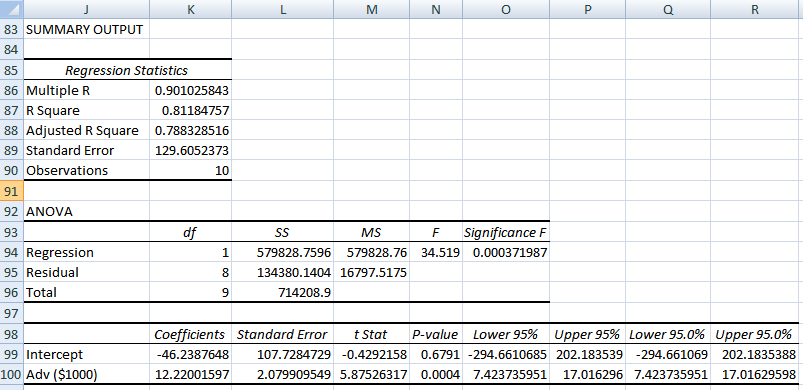
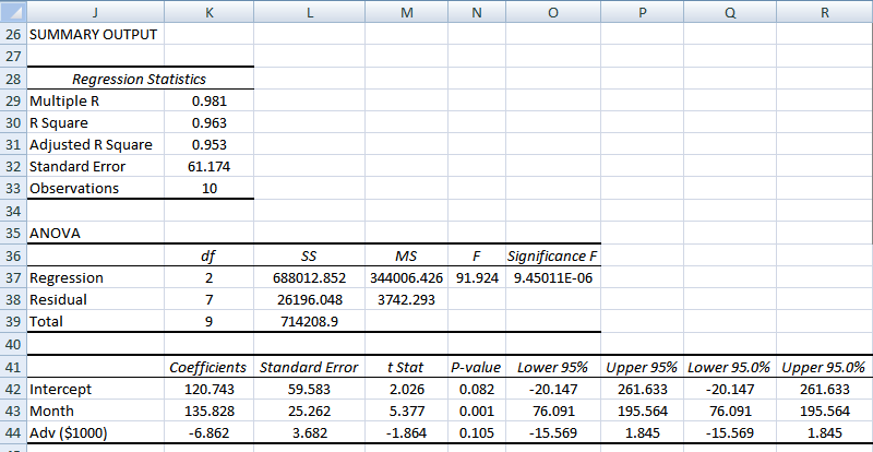
4 e. Click any data point on the scatter plots for Month and Sales, or Adv and Sales, select Add Trendline / Display equations & Display R-Squared value on the charts. The Y and Xs are renamed to Month, Adv and Sales, respectively, for the regression lines. 4. What are the values of b 0, b 1, and b 2, and what is the estimated regression function? The values of b 0, b 1, and b 2 are , and , respectively as given in the Table above. 5. What are the meaning of b 0, b 1, and b 2? When in Month=0, and Adv=0, the Sales = b 0 =$ , b 1 =$ shows the marginal change (increase or decrease) of $ in Sales when the variable Month changes one unit (increase or decrease) while keep no change for Adv., b 2 = shows the marginal change (decrease or increase) of $6.862 in Sales (Y) when the amount of the variable Adv$ (X 2 ) incrementally changes (increases or decreases ONE unit) while keep no change for Month. 6. Use Excel@ =RSQ(Array Y,Array X) to compute the coefficient of Determination R 2 of the regression line for the data, and interpret the meaning of R 2 for the data? (Regression.xls/Reg1) For the regression line for Month versus Sales, R 2 = 94.5% means 94.5% of the total variations in Sales are counted for or explained and 5.5% of the total variations are not counted for or not explained by the regression line between Month and Sales. For the regression line for Adv versus Sales, R 2 = 81.18% means 81.18% of the total variations in Sales are counted for or explained and 18.82%% of the total variations are not counted for or not explained by the regression line between the Adv and Sales. 7. For the Summary Table from Data/Data Analysis, answer the following questions: a. R 2, Adjusted R 2, Number of Observations, b 0, b 1, p-value for b 0, p-value for b 1. The values are as labeled in the above table from Regression.xls/Reg1SO. b. Use the p-value approach to test the population parameters β 0, β 1 and β 2 with the p-values from the Summary Output of Data Analysis/Regression, and state your conclusion. Assume the significance coefficient α = (Regression.xls/Reg1SOa) Hypothesis Test for β 0 : i. What are the H 0 and H 1? H 0 : β 0 = 0 and H 1 : β 0 0 ii. What are the decision rules? Decision Rules with p-value Approach: If p-value α (significance coefficient), then conclude H 0 or β 0 = 0; Otherwise, if p-value < α, then conclude H a, or β 0 0. iii. What is the conclusion? The p-value for β 0 = as given in the Summary Output, it is greater than α = 0.05, therefore, we conclude H 0 : β 0 = 0 or fail to reject H 0, i.e., we should not include the Y intercept term in the regression model for Sales. 4

5 Hypothesis Test for β 1 (Month): i. What are the H 0 and H 1? H 0 : β 1 = 0 and H 1 : β 1 0 ii. What are the decision rules? Decision Rules with p-value Approach: If p-value α (significance coefficient), then conclude H 0 or β 1 = 0; Otherwise, if p-value < α, then conclude H a, or β 1 0. iii. What is the conclusion? The p-value for β 1 = as given in the Summary Output, it is less than α = 0.05, therefore, we conclude H 1 : β 1 0 or reject reject H 0, i.e., we should include the variable Month in the regression model for Sales. Hypothesis Test for β 2 (Adv): i. What are the H 0 and H 1? H 0 : β 2 = 0 and H 1 : β 2 0 ii. What are the decision rules? Decision Rules with p-value Approach: If p-value α (significance coefficient), then conclude H 0 or β 2 = 0; Otherwise, if p-value < α, then conclude H a, or β 2 0. iii. What is the conclusion? The p-value for β 2 = as given in the Summary Output, it is greater than α = 0.05, therefore, we conclude H 0 : β 0 = 0 or fail to reject H 0, i.e., we should not include the variable Adv in the regression model for Sales. Therefore the final regression model for Sales becomes: Sales = b 1 (Month). We have to go through additional procedures below to find out the value of b 1 when the Y intercept b 0 is zero. For reference: Decision Rules with Confidence Interval Approach: If the given CI spans zero (with zero as part of CI), conclude H 0 Otherwise, if the given CI does not span zero, then conclude H a 8. What are the forecasts for the next two years (11 to 12) with the regression line? Because the hypothesis tests reveal only β 1 is significant and should be included in the model, we further run the models with Adv only and Month only with the results in the following two tables. (Regression.xls/Reg1SOb) (Regression.xls/Reg1SOc) 5

6 The results reveal that the Y intercept terms on both cases are not significant, thus should not be included in the model, the variables Month and Adv, each is significant to model the Sales by itself. We therefore decide to use Month only as recommended in the procedure 7.b above. To find out the value of b 1 without b 0 with the variable Month only, we need to rerun the Data/Data Analysis/Regression with the option of Constant is Zero as given below. (Regression.xls/Reg1) The final Summary Output Table is given in Regression.xls/Reg1SOd) (Regression.xls/Reg1SOd) a. Manually compute the forecasts with the b 0,b 1 and b 2 from the previous results Sales (Month=11) = * 11 (Month) = $ in Excel@ =Reg1SOd!$B$18*'Reg1'!A12 Sales (Month=12) = * 12 (Month) = $ in Excel@ =Reg1SOd!$B$18*'Reg1'!A13 In this case, Excel@ = TREND() cannot be used to forecast future Sales. The following procedures are used to show how to use =TREND() to forecast Sales when b 0, b 1, and b 2 are all included in the model for Sales. We use TREND2 to represent the forecasts developed with =TREND() with both Month and Adv in the model for Sales. Assume the Adv = 35 for Month = 11, and Adv = 45 for Month = 12. Please note the use of Absolute Address in =TREND(). 6

7 b. Use =TREND(Y-RANGE,X-RANGE,X-VALUE) (Regression.xls/Reg1) c. What is the assumption you made when you develop forecasts for the next two years? The crucial assumption made for using linear regression is that the linear trend for Sales is going to continue in Months 11 and 12 with the b 2 = Thus any forecasts made outside out the original ranges of independent variable Xs in the historical data may not be valid. 9. What is the difference between standard error (S e ) and the standard prediction error (S p )? Standard Error of Estimate ( S e ): = = ( ) 1 = = = = S e measures the variation of the actual data around the estimated regression line, where k is the number of independent variables in the model. Standard prediction error (S p ): thus the S p is always larger than S e. (1 α)% Prediction Interval for individual response Y: = ( ) ( ) = + and ± ( ;) 7

8 (Regression.xls/Reg1SOd) The following results are in Regsssion.xls/Reg What is the margin of error for an approximate 95% prediction interval individual response for Month=11? The margin of prediction error for Month=11 is What is the 95% mean prediction interval for Month=11? Lw Lmt of 95% Mean Pred CI for Month= Up Lmt of 95% Mean Pred CI for Month= What is the 95% prediction intervals individual response for the Month = 11? Lw Lmt of 95% Pred CI for Month= Up Lmt of 95% Pred CI for Month= Appro Lw Lmt of 95% Pred CI for Month = Appro Up Lmt of 95% Pred CI for Month = 11 8

9 (Regression.xls/Reg2) 9

10 Topics to be covered: 1. Regression as a method in business analytics =(,,, )+ a. Simple Linear Regression (SLP) =()+ or = + + and and as estimates for, = + to min = ( ) = ( + ) and the method of least squares b. Simple Linear Regression with Time as Independent Variable =()+ or = + + c. Multiple Regression =(,,, )+, where f(.) describes systematic variations and ε describers unsystematic variations of the system. 2. Assumptions for Regression 10

11 3. Using to do Regression analysis = + Decomposition of the Total Error: =( )+( ) ( ) =( ) +( ) TSS = ESS + RSS Or Total Sum of Squared Errors (TSS) = Error Sum of Squares (ESS) + Regression Sum of Squares (RSS) = =1, and 0 R2 1 R 2 refers to the percentage of the total variation of Y around its mean that is explained or counted for by the estimated regression line or how well the regression line fits the data. 1-R 2 is the percentage of the total variation of Y around its mean that is unexplained or uncounted for by the regression line. Equations to compute b 0 and b 1 : = = ( )( ) ( ) = = 11

12 Standard error of estimate versus Standard prediction error: Standard Error of Estimate ( S e ), the Rule of Thumb and Standard Prediction Error (S p ): = = ( ) 1 = = = 1 Se measures the variation of the actual data around the estimated regression line, where k is the number of independent variables in the model. The rule of thumb: 68%, 95% and 99.7% of the observations are within ±1 S e, ±2 S e and ±3 S e or the approximate 95% Confidence Interval for individual can be roughly estimated as ±2 Standard prediction error (S p ): thus the S p is always larger than S e. = ( ) ( ) (1 α)% Prediction Interval for individual response Y: = + and ± ( ;) For α = 0.10, 1 α/2 = 0.95, the ( ;) = TINV(1-α,n-2)=TINV(0.10,n-2). Please note, TINV assumes two tailed case. (1 α)% Confidence Interval for the mean of Y at the given point of X: For multiple Regressions: =1 1 1 ± ( ;) 1 + ( ) ( ) 12

13 Statistical Tests for β 0, β 1,, β k with F-Statistic, p-value and t-statistic: How to get the regression line in Excel@? o =INTERCEPT(Y-RANGE,X-RANGE) and =SLOPE(Y-RANGE,X-RANGE) o =TREND(Y-RANGE,X-RANGE,X-VALUE) o In Excel@ Data/Data Analysis/Regression o In Excel@, insert/scatter plot, Click any data points in the scatter plot, select Add Trendline / Display equations & Display R-Squared value on chart o Use Excel Solver to Minimize ESS What are the meanings of the slope(β 1, β n ) and the intercept(β 0 )? Meanings of b 0 and b 1 : o b 0 is the intercept or Y value as X = 0 (e.g. Fixed cost) o b 1 is the slope or marginal change in Y with unit change in X o b 1 is similar to the slope. However, since it is calculated with the variability of the data in mind, its formulation is not as straight-forward as our usual notion of slope. How to statistically test whither β 0, β 1, β n equals zero (in the Null Hypothesis H 0 )? o Use the p-value approach because p-values will be in Summary Output. Decision Rule is: if p-value is less than α value (Type I error, not the one in Exponential smoothing forecasting), then conclude β 0, β 1, β n not equal to zero. o Only include b 0, b 1,, b n in the equation if β 0, β 1, β n not equal to zero. Exclude the zero ones How to interpret R 2? Percentage of total variations explained by the regression line. (1-R2) is the percentage of total variations not explained by the regression line. How to develop forecasts with given b 0, b 1,, b n? o = + + for each value of X and could be X 1, X 2,, and X n. 13

14 o Predictions made using an estimated regression function may have little or no validity for values of the independent variables that are substantially different from those represented in the sample. o Avoid multicollinearity when more than one independent variables are in the model. How to estimate the prediction confidence intervals? o The approximate prediction confidence interval, ±2, where S e is the standard error given in the Summary Output beneath the Adjusted R 2. o The prediction confidence interval for the mean response is given by ± o The prediction confidence interval for individual response is given by ±, where S p is the standard prediction error and S p is always larger than S e. How to develop forecasting with Trend, Seasonal and Random components with the multiplicative model Y = T.S.I? o Use regression or centered moving average to take out the trend component detrend o Use S.I = Y/T to get the percentage of Trend o Compute Seasonal Relatives by average the percentages of Trend in the same season o Adjust the Seasonal Relatives to the whole number (Quarterly seasonality in a year will be 4, Weekly seasonality will be 7, etc.) to get the Seasonal Index. o Attached the Seasonal Index to each season o Develop the trend forecast with regression or other methods o Use the Seasonal Index to multiply the previous forecasts to develop the final seasonally adjusted forecast. 14

15 Sales ($1000) y = 12.22x R² = Adv ($1000) Sales ($1000) y = x R² = Month Simple Linear Regression with Time as Independent Variable =()+ or = + + and = + 15

16 16

17 17

18 Meanings of Regression Summary Output R 2 Adjusted R 2 S e n SSR SSE SST MSR MSE p-value Regression b 0 Confidence Intervals for b 0, b 1 and b 2 b 1 b 2 S b0 Sb1 Sb2 p-value to test b 1 = 0 p-value to test b 0 = 0 p-value to test b 2 = 0 Decision Rules with p-value Approach: If p-value α (significance), then conclude H 0 or b 0, b 1 or b 2 is zero Otherwise, if p-value < α, then conclude H a or b 0, b 1 or b 2 is not zero Decision Rules with Confidence Interval Approach: If the given CI spans zero (with zero as part of CI), conclude H 0 Otherwise, if the given CI does not span zero, then conclude H a 18