An Introduction to Information Theory

Transcription

1 An Introduction to Information Theory Carlton Downey November 12, 2013

2 INTRODUCTION Today s recitation will be an introduction to Information Theory Information theory studies the quantification of Information Compression Transmission Error Correction Gambling Founded by Claude Shannon in 1948 by his classic paper A Mathematical Theory of Communication It is an area of mathematics which I think is particularly elegant

3 OUTLINE Motivation Information Entropy Marginal Entropy Joint Entropy Conditional Entropy Mutual Information Compressing Information Prefix Codes KL Divergence

5 MOTIVATION: CASINO You re at a casino You can bet on coins, dice, or roulette Coins = 2 possible outcomes. Pays 2:1 Dice = 6 possible outcomes. Pays 6:1 roulette = 36 possible outcomes. Pays 36:1 Suppose you can predict the outcome of a single coin toss/dice roll/roulette spin. Which would you choose?

6 MOTIVATION: CASINO You re at a casino You can bet on coins, dice, or roulette Coins = 2 possible outcomes. Pays 2:1 Dice = 6 possible outcomes. Pays 6:1 roulette = 36 possible outcomes. Pays 36:1 Suppose you can predict the outcome of a single coin toss/dice roll/roulette spin. Which would you choose? Roulette. But why? these are all fair games

7 MOTIVATION: CASINO You re at a casino You can bet on coins, dice, or roulette Coins = 2 possible outcomes. Pays 2:1 Dice = 6 possible outcomes. Pays 6:1 roulette = 36 possible outcomes. Pays 36:1 Suppose you can predict the outcome of a single coin toss/dice roll/roulette spin. Which would you choose? Roulette. But why? these are all fair games Answer: Roulette provides us with the most Information

8 MOTIVATION: COIN TOSS Consider two coins: Fair coin CF with P(H) = 0.5, P(T) = 0.5 Bent coin CB with P(H) = 0.99, P(T) = 0.01 Suppose we flip both coins, and they both land heads Intuitively we are more surprised or Informed by first outcome. We know C B is almost certain to land heads, so the knowledge that it lands heads provides us with very little information.

9 MOTIVATION: COMPRESSION Suppose we observe a sequence of events: Coin tosses Words in a language notes in a song etc. We want to record the sequence of events in the smallest possible space. In other words we want the shortest representation which preserves all information. Another way to think about this: How much information does the sequence of events actually contain?

10 MOTIVATION: COMPRESSION To be concrete, consider the problem of recording coin tosses in unary. T, T, T, T, H Approach 1: H T , 00, 00, 00, 0 We used 9 characters

11 MOTIVATION: COMPRESSION To be concrete, consider the problem of recording coin tosses in unary. T, T, T, T, H Approach 2: H T , 0, 0, 0, 00 We used 6 characters

12 MOTIVATION: COMPRESSION Frequently occuring events should have short encodings We see this in english with words such as a, the, and, etc. We want to maximise the information-per-character seeing common events provides little information seeing uncommon events provides a lot of information

14 INFORMATION Let X be a random variable with distribution p(x). We want to quantify the information provided by each possible outcome. Specifically we want a function which maps the probability of an event p(x) to the information I(x) Our metric I(x) should have the following properties: I(x i ) 0 i. I(x 1 ) > I(x 2 ) if p(x 1 ) < p(x 2 ) I(x1, x 2 ) = I(x 1 ) + I(x 2 )

15 INFORMATION I(x) = f (p(x)) We want f () such that I(x 1, x 2 ) = I(x 1 ) + I(x 2 ) We know p(x 1, x 2 ) = p(x 1 )p(x 2 ) The only function with this property is log(): log(ab) = log(a) + log(b) Hence we define: I(X) = log( 1 p(x) )

16 INFORMATION: COIN Fair Coin: h t I(h) = log( ) = log(2) = 1 I(t) = log( ) = log(2) = 1

17 INFORMATION: COIN Bent Coin: h t I(h) = log( ) = log(4) = 2 I(t) = log( 1 ) = log(1.33) =

18 INFORMATION: COIN Really Bent Coin: h t I(h) = log( 1 ) = log(100) = I(t) = log( 1 ) = log(1.01) =

19 INFORMATION: TWO EVENTS Question: How much information do we get from observing two events? 1 I(x 1, x 2 ) = log( p(x 1, x 2 ) ) Answer: Information sums! 1 = log( p(x 1 )p(x 2 ) ) 1 1 = log( p(x 1 ) p(x 2 ) ) 1 = log( p(x 1 ) ) + log( 1 p(x 2 ) ) = I(x 1 ) + I(x 2 )

20 INFORMATION IS ADDITIVE I(k fair coin tosses) = log 1 = k bits 1/2 k So: Random word from a 100,000 word vocabulary: I(word) = log(100, 000) = bits A 1000 word document from same source: I(documents) = 16,610 bits A 480 pixel, 16-greyscale video picture: I(picture) = 307, 200 log(16) = 1,228,800 bits A picture is worth (a lot more than) 1000 words! In reality this is a gross overestimate

21 INFORMATION: TWO COINS Bent Coin: x h t p(x) I(x) I(hh) = I(h) + I(h) = 4 I(ht) = I(h) + I(t) = 2.42 I(th) = I(t) + I(h) = 2.42 I(th) = I(t) + I(t) = 0.84

22 INFORMATION: TWO COINS Bent Coin Twice: hh ht th tt I(hh) = 1 log( ) = log(4) = 4 I(ht) = 1 log( ) = log(4) = I(th) = 1 log( ) = log(4) = I(tt) = 1 log( ) = log(4) =

24 ENTROPY Suppose we have a sequence of observations of a random variable X. A natural question to ask is what is the average amount of information per observation. This quantitity is called the Entropy and denoted H(X) 1 H(X) = E[I(X)] = E[log( p(x) )]

25 ENTROPY Information is associated with an event - heads, tails, etc. Entropy is associated with a distribution over events - p(x).

26 ENTROPY: COIN Fair Coin: x h t p(x) I(x) 1 1 H(X) = E[I(X)] = p(x i )I(X) i = p(h)i(h) + p(t)i(t) = = 1

27 ENTROPY: COIN Bent Coin: x h t p(x) I(x) H(X) = E[I(X)] = p(x i )I(X) i = p(h)i(h) + p(t)i(t) = = 0.85

28 ENTROPY: COIN Very Bent Coin: x h t p(x) I(x) H(X) = E[I(X)] = p(x i )I(X) i = p(h)i(h) + p(t)i(t) = = 0.08

29 ENTROPY: ALL COINS

30 ENTROPY: ALL COINS H(P) = p log 1 p + (1 p) log 1 1 p

31 ALTERNATIVE EXPLANATIONS OF ENTROPY H(S) = i p i log 1 p i Average amount of information provided per event Average amount of surprise when observing a event Uncertainty an observer has before seeing the event Average number of bits needed to communicate each event

32 THE ENTROPY OF ENGLISH 27 Characters (A-Z, space) 100,000 words (average 5.5 characters each) Assuming independence between successive characters: Uniform character distribution: log(27) = 4.75 bits/characters True character distribution: 4.03 bits/character Assuming independence between successive words: Uniform word distribution: log(100,000) 6.5 = 2.55 bits/character True word distribution: = 1.45 bits/character True Entropy of English is much lower

33 TYPES OF ENTROPY There are 3 Types of Entropy Marginal Entropy Joint Entropy Conditional Entropy We will now define these quantities, and study how they are related.

34 MARGINAL ENTROPY A single random variable X has a Marginal Distribution p(x) This distribution has an associated Marginal Entropy H(X) = i p(x i ) log 1 p(x i ) Marginal entropy is the average information provided by observing a variable X

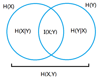
35 JOINT ENTROPY Two or more random variables X, Y have a Joint Distribution p(x, Y) This distribution has an associated Joint Entropy H(X, Y) = i 1 p(x i, y j ) log p(x i, y j ) j Marginal entropy is the average total information provided by observing two variables X, Y

36 CONDITIONAL ENTROPY Two random variables X, Y also have two Conditional Distributions p(x Y) and P(Y X) These distributions have associated Conditional Entropys H(X Y) = j = j = i p(y j )H(X y j ) p(y j ) p(x i y j ) log i p(x i, y j ) log j 1 p(x i y j ) 1 p(x i y j ) Conditional entropy is the average additional information provided by observing X, given we already observed Y

37 TYPES OF ENTROPY: SUMMARY Entropy: Average information gained by observing a single variable Joint Entropy: Average total information gained by observing two or more variables Conditional Entropy: Average additional information gained by observing a new variable

38 ENTROPY RELATIONSHIPS

39 RELATIONSHIP: H(X, Y) = H(X) + H(Y X) H(X, Y) = 1 p(x i, y j ) log( p(x i, y j ) ) i,j = 1 p(x i, y j ) log( p(y j x i )p(x i ) ) i,j = [ ] 1 p(x i, y j ) log( p(x i ) ) + log( 1 p(y j x i ) ) i,j = 1 p(x i ) log( p(x i ) ) + 1 p(x i, y j ) log( p(y j x i ) ) i i = H(X) + H(Y X)

40 RELATIONSHIP: H(X, Y) H(X) + H(Y) We know H(X, Y) = H(X) + H(Y X) Therefore we need only show H(Y X) H(Y) This makes sense, knowing X can only decrease the addition information provided by Y.

41 RELATIONSHIP: H(X, Y) H(X) + H(Y) We know H(X, Y) = H(X) + H(Y X) Therefore we need only show H(Y X) H(Y) This makes sense, knowing X can only decrease the addition information provided by Y. Proof? Possible homework =)

42 ENTROPY RELATIONSHIPS

43 MUTUAL INFORMATION The Mutual Information I(X; Y) is defined as: I(X; Y) = H(X) H(X Y) The mutual information is the amount of information shared by X and Y. It is a measure of how much X tells us about Y, and vice versa. If X and Y are independent then I(X; Y) = 0, because X tells us nothing about Y and vice versa. If X = Y then I(X; Y) = H(X) = H(Y). X tells us everything about Y and vice versa.

44 EXAMPLE Marginal Distribution: X sun rain Y hot cold P(X) P(Y) Conditional Distribution: Y hot cold P(Y X = sun) Y hot cold P(Y X = rain) Joint Distribution: hot cold sun rain

45 EXAMPLE: MARGINAL ENTROPY Marginal Distribution: X sun rain P(X) H(X) = i 1 p(x i ) log( p(x i ) ) = 0.6 log( 1 1 ) log( ) = 0.97

46 EXAMPLE: JOINT ENTROPY Joint Distribution: hot cold sun rain H(X) = i,j 1 p(x i, y i ) log( p(x i, y i ) ) = 0.48 log( ) + 2 = 1.76 [ 0.12 log( 1 ] 0.12 ) log( )

47 EXAMPLE: CONDITIONAL ENTROPY Joint Distribution: hot cold sun rain Conditional Distribution: Y hot cold P(Y X = sun) Y hot cold P(Y X = rain) H(Y X) = i,j 1 p(x i, x j ) log( p(y i x i ) ) = 0.48 log( ) log( ) log( ) log( ) = 0.79

48 EXAMPLE: SUMMARY Results: H(X) = H(Y) = 0.97 H(X, Y) = 1.76 H(Y X) = 0.79 I(X; Y) = H(Y) H(Y X) = 0.18 Note that H(X, Y) = H(X) + H(Y X) as required. Interpreting the Results: I(X; Y) > 0, therefore X tells us something about Y and vice versa H(Y X) > 0, therefore X doesn t tell us everything about Y

49 MOTIVATION RECAP Gambling: Coins vs. Dice vs. Roulette Prediction: Bent Coin vs. Fair Coin Compression: How to best record a sequence of events

51 PREFIX CODES Compression maps events to code words We already saw an example when we mapped coin tosses to unary numbers We want mapping which generates short encodings One good way of doing this is prefix codes

52 PREFIX CODES Encoding where no code word is a prefix of any other code word. Event a b c d Example: Code Word Previously we reserved 0 as a separator If we use a prefix code we do not need a separator symbol = bbaacdcd

53 DISTRIBUTION AS PREFIX CODES Every probability distribution can be thought of as specifying an encoding via the Information I(X) Map each event x i to a word of length I(x i ) Table: Fair Coin X h t P(X) I(X) 1 1 code(x) 1 0

54 DISTRIBUTION AS PREFIX CODES Every probability distribution can be thought of as specifying an encoding via the Information I(X) Map each event x i to a word of length I(x i ) Table: Fair 4-Sided Dice X P(X) I(X) code(x)

55 DISTRIBUTION AS PREFIX CODES Every probability distribution can be thought of as specifying an encoding via the Information I(X) Map each event x i to a word of length I(x i ) Table: Bent 4-Sided Dice X P(X) I(X) code(x)

56 DISTRIBUTION AS PREFIX CODES Prefix codes built from the distribution are optimal Information is contained in the smallest possible number of characters Entropy is maximized Encoding is not always this obvious. e.g. How to encode a bent coin Question: If use a different (suboptimal) encoding, how many extra characters do I need

57 KL DIVERGENCE

58 KL DIVERGENCE The expected number of additional bits required to encode p using q, rather than p using p. D KL (p q) = i = i p(x i ) codeq (x i ) p(x i ) codep (x i ) p(x i )I q (x i ) i i p(x i )I p (x i ) = i 1 p(x i ) log( q(x i ) ) i 1 p(x i ) log( p(x i ) )

59 KL DIVERGENCE The KL Divergence is a measure of the Dissimilarity of two distributions If p and q are similar, then KL(p q) will be small. Common events in p will be common events in q This means they will still have short code words If p and q are dissimilar, then KL(p q) will be large. Common events in p may be uncommon events in q This means commonly occuring events might be given long codewords

60 SUMMARY Motivation Information Entropy Marginal Entropy Joint Entropy Conditional Entropy Mutual Information Compressing Information Prefix Codes KL Divergence