Comparison of Five Modeling Approaches to Quantify and Estimate the Effect of Clouds on the Radiation Amplification...

Transcription

1 See discussions, stats, and author profiles for this publication at: Comparison of Five Modeling Approaches to Quantify and Estimate Effect of Clouds on Radiation Amplification... Article in Atmosphere August 2017 DOI: /atmos CITATIONS 0 READS 14 1 author: Eric Steven Hall United States Environmental Protection Agency 56 PUBLICATIONS 31 CITATIONS SEE PROFILE Some of authors of this publication are also working on se related projects: Multi-Sector Sustainability Browser (MSSB) View project All content following this page was uploaded by Eric Steven Hall on 25 August The user has requested enhancement of downloaded file.

2 atmosphere Article Comparison of Five Modeling Approaches to Quantify and Estimate Effect of Clouds on Radiation Amplification Factor (RAF) for Solar Ultraviolet Radiation Eric S. Hall ID Exposure Research Laboratory, Office of Research and Development, US Environmental Protection Agency, Mail Drop E205-03, 109 T. W. Alexander Drive, Research Triangle Park, NC 27711, USA; Received: 16 June 2017; Accepted: 16 August 2017; Published: 18 August 2017 Abstract: A generally accepted value for Radiation Amplification Factor (RAF), with respect to erymal action spectrum for sunburn of human skin, is 1.1, indicating that a 1.0% increase in stratospheric ozone leads to a 1.1% decrease in biologically damaging UV radiation in erymal action spectrum reaching Earth. The RAF is used to quantify non-linear change in biologically damaging UV radiation in erymal action spectrum as a function of total column ozone (O 3 ). Spectrophotometer measurements recorded at ten US monitoring sites were used in this analysis, and over 71,000 total UVR measurement scans of sky were collected at those 10 sites between 1998 and 2000 to assess RAF value. This UVR dataset was examined to determine specific impact of clouds on RAF. Five de novo modeling approaches were used on dataset, and calculated RAF values ranged from a low of 0.80 to a high of Keywords: Radiation Amplification Factor (RAF); solar zenith angle (SZA); Dobson Unit (DU); ultraviolet (UV); ultraviolet radiation (UVR); cloudiness 1. Introduction The Radiation Amplification Factor (RAF) is defined as measured percentage change in ultraviolet (UV) irradiance for each one-percent change in total column ozone [1]. Understanding variations in measured ultraviolet radiation (UVR) over time, along with associated RAF values, assists health scientists in determining risks associated with UVR exposure through RAF for individuals and environment [2]. Exposure to ultraviolet radiation (UVR) poses risks to both humans and environment, refore a number of national and international government, industrial, and university research organizations initiated programs to measure amount of UVR reaching Earth s surface, since stratospheric ozone affects amount of UVR reaching Earth. The United States Environmental Protection Agency (US EPA) conducted a research program from 1996 to 2004 to measure ultraviolet radiation (UVR) at 21 network sites throughout continental US, Alaska, Hawaii and US Virgin Islands (St. John) under all wear conditions. The US EPA Exposure Research Laboratory (NERL) developed UV Radiation Research Program to measure intensity of UVR at distinct locations throughout US that differed in spatial location, geography, climate, altitude, and ecology. The three major categories of research-grade instruments that have been used to detect UVR are broadband, narrowband, and spectral. NERL chose spectral UVR monitors called Brewer Spectrophotometers. When operated within a disciplined calibration and maintenance program, instruments precisely measure UVR levels through a well-defined portion of electromagnetic spectrum wavelengths (286.5 nm to 363 nm). Maintaining long-term calibration Atmosphere 2017, 8, 153; doi: /atmos

3 Atmosphere 2017, 8, of 33 of spectral instruments requires great effort. They are more expensive to operate in comparison to broadband or narrowband instruments, because y require highly skilled operators. The Brewer instruments were calibrated for biologically damaging UV radiation in erymal action spectrum at each of 21 sites using a secondary (travelling) standard lamp traceable to a primary (stationary) Institute of Standards and Technology (NIST) 1000-W lamp. The calibrations were performed by scientists at University of Georgia at Ans (UGA) UV Monitoring Center (NUVMC) on an annual basis. The calibrated Brewer data used a daily temporal response (estimated) based on annual calibration. In addition, independent quality assurance audits of Brewers were performed by scientists from Oceanic and Atmospheric Administration (NOAA) Central UV Calibration Facility (CUCF). Quarterly checks on transfer of calibration standard from NIST 1000-W lamp to traveling secondary standard were performed at NUVMC. The response function of each instrument was calculated daily from a linear interpolation between two (temporally) closest response functions. Brewer data were corrected for dark count, dead time, and stray light. Clouds affect relative absorption/reflectance of UVR. Transmittance of UVR through clouds is shown to be wavelength dependent, ranging from 45% in UV-A region to 60% in UV-B region as stated in Chapter 4, page 105 of [3]. Cloud features known to affect transmission of UVR include cloud amount and coverage (e.g., percentage of sky covered), particle size distribution, cloud spatial and temporal variability, season, location, etc., [4]. Realistically, clouds can eir increase or decrease amount of UVR at surface [5]. Due to unpredictable nature of clouds, extent of cloudiness (percent clearness) of sky had to be determined for this analysis in a consistent, logically defensible manner, to determine effect of clouds on Radiation Amplification Factor (RAF). Using a consistent definition of cloudiness, results seem to indicate that average RAF values generally approximate 1.1 at se 10 sites (two urban sites and eight US Parks sites), and that total column ozone (O 3 ) and solar zenith angle (SZA) are most important parameters in determining biologically damaging UV radiation in erymal action spectrum reaching Earth s surface. Five modeling approaches, labelled A, B, C, D, and E, were used to estimate impact of clouds on biologically damaging UV radiation in erymal action spectrum Development of EPA s UVR Monitoring Network In early 1990s, EPA s Office of Research and Development (ORD) originally designed a UVR monitoring network of five to seven sites principally in urban areas, with a few pristine rural sites for monitoring background UVR levels. The EPA s role in UVR research was to monitor in urban areas. The United States Department of Agriculture (USDA) was responsible for monitoring UVR in rural areas. The focus of EPA s original UVR network design was shifted in In September 1996, US EPA and US Parks Service (NPS), of US Department of Interior (DOI), signed an Interagency Agreement (IAG) to cooperate on a program of long-term monitoring of environmental stressors, including UVR, at 21 separate locations throughout United States. When NPS sites were added to network, it greatly expanded EPA s UVR monitoring program. The EPA s UVR Monitoring Network facilitated research on observed effects that environmental stressors, including UVR, pose on various ecosystems and on human health. The 21 EPA UVR monitoring sites (displayed in Figure 1) were located throughout continental United States, Alaska (Denali Park), Hawaii (Hawaii Volcanoes Park) and US Virgin Islands (Virgin Islands Park, St. Johns, VI). Fourteen of sites were located in US Parks, and seven sites were located in urban settings. Data collected from 21 sites was processed through a quality assurance protocol to ensure proper characterization of UVR intensities measured at each site.

4 4. 5. Evaluate human and ecosystem/environmental exposure to surface UVR across US. Assess impact of changes in stratospheric ozone and tropospheric pollution on biologically damaging UV radiation in erymal action spectrum. 6. Assess effectiveness of control strategies (e.g., Montreal Protocol) designed to reduce amount of greenhouse gases in stratosphere, and increase amount of stratospheric ozone. Atmosphere 2017, 8, of Serve as a component of EPA s Environmental Monitoring Strategy. Figure 1. 1.Location in Environmental EnvironmentalProtection Protection Agency (EPA) Figure LocationofofBrewer BrewerSpectrophotometers Spectrophotometers in Agency (EPA) ultraviolet radiation (UVR) ultraviolet radiation (UVR)Monitoring MonitoringNetwork. Network. During development phase ofinstruments EPA s UVR Monitoring Network, experimental design The 21 deployed UVR monitoring measured full sky UV radiation. These instruments and site planned test specific hyposes, which fulfilled stated research tracked selection sun and were monitored to variation in solar energy throughout day. The instruments objectives listed above. Sites were selected which provided UVR data for a variety of conditions (e.g.,[6]. measured UVR at wavelengths between nm and 363 nm in 0.5 nm wavelength increments high and low elevation, high and low cloud cover, high and low air pollution levels, latitude and Therefore, each scan produced 154 discrete wavelength values for which UVR would be measured. longitude variation, ecosystem variations [fresh and marine water], etc.). The EPA decided that The data collected at each network site could n be used to calculate both dose and dose rate network would consist of spectral UVR monitors so that researchers could determine what key of UVR received at Earth s surface at various times throughout day. The instruments were factors caused changes in UVR levels, e.g., changes in stratospheric ozone composition, tropospheric mounted on an azimuth tracker and tripod unit connected to a desktop computer running Disk changes like cloud cover or pollution (e.g., black carbon, and particulate matter), etc. A secondary Operating System (DOS) and GWTM Basic Software for instrument control. benefit of spectral UVR data is that data on UV spectrum can be compared with data on The major objectives of EPA s UVR Monitoring Network were to: human and ecological disease incidence and geographic distribution. 1. Improve understanding of nature and intensity of UVR reaching Earth s surface. 2. Characterize physical and chemical parameters that modify UVR flux. Obtain better estimates of UVR exposures at multiple times, locations, meteorological conditions, 3. altitudes, terrain characteristics, topologies, and air pollution conditions. 4. Evaluate human and ecosystem/environmental exposure to surface UVR across US. 5. Assess impact of changes in stratospheric ozone and tropospheric pollution on biologically damaging UV radiation in erymal action spectrum. 6. Assess effectiveness of control strategies (e.g., Montreal Protocol) designed to reduce amount of greenhouse gases in stratosphere, and increase amount of stratospheric ozone. 7. Serve as a component of EPA s Environmental Monitoring Strategy. During development phase of EPA s UVR Monitoring Network, experimental design and site selection were planned to test specific hyposes, which fulfilled stated research objectives listed above. Sites were selected which provided UVR data for a variety of conditions (e.g., high and low elevation, high and low cloud cover, high and low air pollution levels, latitude and longitude variation, ecosystem variations [fresh and marine water], etc.). The EPA decided that network

5 Atmosphere 2017, 8, of 33 would consist of spectral UVR monitors so that researchers could determine what key factors caused changes in UVR levels, e.g., changes in stratospheric ozone composition, tropospheric changes like cloud cover or pollution (e.g., black carbon, and particulate matter), etc. A secondary benefit of spectral UVR data is that data on UV spectrum can be compared with data on human and ecological disease incidence and geographic distribution. The first (experimental) site in EPA s UVR Monitoring Network at Research Triangle Park, North Carolina, began initial operation in The UVR data collected from EPA s UVR Monitoring Network was processed through a Level-1 data quality assurance algorithm to ensure proper characterization of biologically damaging UV radiation intensities at each measured wavelength (for each instrument), and data in this study is designated as Level-1 corrected data [7]. The Level 1 algorithm included corrections for calibration drift of instruments, cosine response, and temperature effects. Once raw UVR monitoring data is run through L1 algorithm, acceptance or rejection of a scan measurement value is based on number of successful instrument scans during a given day and range of L1-corrected biologically damaging UV radiation values. During term of monitoring program, a total of 40,474 site-days worth of UVR data was collected through EPA s UVR Monitoring Network, with 35,811 site-days being usable for analysis (88.5%). The network collected over 500,000 individual measurements (scans) of UVR data during program [8] Importance of UVR Monitoring The sun is a near-ideal blackbody radiator with a temperature of 6000 degrees (6000 ) Kelvin, emitting electromagnetic radiation in a wide and continuous spectral distribution; however, spectral instruments with photo diode arrays or charge-coupled devices (CCDs) can record entire spectrum simultaneously [9]. The wavelength peak in its emission curve resides in visible wavelength region. Although sun emits a tremendous amount of solar energy on a daily basis, Earth captures only a small portion of sun s radiant energy, approximate 1370 Watts per meter squared (W/m 2 ) per day [10]. The energy in UV-A portion of electromagnetic spectrum is approximately 6.3% of total solar energy received at edge of Earth s atmosphere on a daily basis (wavelengths: nm), while UV-B (wavelengths: nm), and UV-C (wavelengths: nm) portions represent 1.5% and 0.5% respectively [11]. Approximately 9% of sun s total solar energy output is in UV spectrum. A high percentage of UV-A reaches Earth s surface (because it is weakly absorbed by atmospheric ozone), but has a low impact on biological systems. UV-B has a greater impact on biological systems than UV-A, but is efficiently screened by ozone. The EPA s UVR monitoring program was conducted in an attempt to detect trends in UVR measurements over time across a wide geographic area Stratospheric Ozone The UVR flux is affected by changes in amount of stratospheric ozone (O 3 ) [12]. The amount of UVR reaching surface of Earth is increased when re is a decrease in amount of stratospheric ozone. One of major factors contributing to a decrease in stratospheric ozone is use of chlorofluorocarbons (CFCs) [13]. CFCs in stratosphere react with ozone through photochemical reactions, which decompose ozone into both monomolecular oxygen and diatomic oxygen species, and although amounts of CFCs used have been significantly reduced, se compounds remain in atmosphere for durations of up to years, contributing to stratospheric ozone reduction [14]. The atmospheric lifetimes of CFCs can be extremely long. CFC-12 (dichlorodifluoromethane), CCl 2 F 2, has an atmospheric lifetime of 100 years, while HCFC-22 (chlorodifluoromethane), CHClF 2, has an atmospheric lifetime of approximately 14.6 years [15]. As stratospheric ozone is reduced, re is less ozone available to absorb UVR, resulting in increased amounts of UVR reaching Earth s surface (holding all or factors constant). Measurement of UVR intensities across United States assisted US policymakers in assessing effectiveness of Montreal Protocol [16], in reducing important

6 Atmosphere 2017, 8, of 33 ozone-depleting substances such as CFCs. Title VI of Clean Air Act [17] also governs protection of stratospheric ozone. 2. Materials and Methods 2.1. Measurement of Ultraviolet (UV) Spectrum Spectral instruments measuring UVR are called scanning spectroradiometers, and se instruments make continuous, spectrally resolved measurements eir across entire electromagnetic spectrum or specific portions of it. Most spectral instruments contain photomultiplier detectors with eir single or double monochromators, where light passes through an initial diffraction grating (usually 1200 or 2400 lines per nm) and through a middle slit which directs light onto a second diffraction grating. The multiple grating configuration minimizes stray light from adjacent wavelengths caused by rapid change of UVR intensity at wavelengths below 320 nm. Multiple diffraction gratings also improve wavelength resolution of scanning spectroradiometers, which can be as low as 0.5 nm [18]. It usually takes several minutes for scanning spectroradiometers to make a single complete scan. The Brewers used in EPA s network were spectral instruments requiring approximately six min to complete a single scan, which introduced temporal variability when clouds pass overhead during a scan period UVR Monitoring Instruments The Brewer is manufactured by Kipp and Zonen (formerly SCI-TEC, Saskatoon, SK, Canada). Figure 2 displays a Mark III Brewer Spectrophotometer that was located in Theodore Roosevelt Park in North Dakota as part of EPA s UVR Monitoring Network. Brewers measure UVR in wavelengths ranging from nm to 363 nm. The measurement resolution for this device is 0.5 nm. This means that 154 separate UVR values are recorded, one value for each wavelength, during each full scan of instrument. Brewers complete 22 to 39 measurement scans per day during summer daylight hours depending on latitude of instrument, with 32 measurement scans being minimum number of ideal scans per day for each instrument during that period. Throughout a full year, expected number of daily scans is approximately Normal instrument repair and maintenance caused by components such as its nickel sulfate filter, photomultiplier tube, bearings, and surges due to lightning strikes and power interruptions reduced instrument availability and subsequently number of scans. The device s scan rate is controlled by ephemeris scheduling software, taking more UVR measurement scans as solar noon approaches at its particular location. The recorded UVR data is stored in computer and archived for post-processing through an algorithm that checks for inconsistent data and or anomalies. The instrument computer controls azimuth tracker which rotates entire Brewer, allowing it to track sun. Brewer software has an ephemeris algorithm, which calculates both azimuth and zenith angles of sun as seen from its (current) location. Brewers accomplish this using its latitude and longitude placement along with its GMT time and date. Angles calculated by ephemeris algorithm along with latitude and longitude are transmitted to both zenith tracker and azimuth tracker systems to properly position Brewer towards sun. Brewers measure biologically damaging UV radiation at each wavelength (spectral irradiance) in instrument s measurement range during each scan of instrument. Spectral irradiance is expressed as power density per unit wavelength (i.e., watts [or milliwatts] per square meter per nanometer [mw/m 2 /nm]). UVR data collected by instruments is important because it helps us understand implications of increased UVR associated with decreasing stratospheric ozone concentrations. The instruments provide accurate UVR measurements of known quality in assessing effectiveness of EPA s stratospheric ozone policies. The data allows scientists to evaluate climatology affecting UVR in environment. The EPA s quality-assured UVR data is posted to a publicly accessible web site: (Last Accessed: 4 August 2017).

7 Atmosphere 2017, 8, of 33 Atmosphere 2017, 8, of 32 Figure 2. Brewer Spectrophotometer located in Theodore Roosevelt Park, North Dakota. Figure 2. Brewer Spectrophotometer located in Theodore Roosevelt Park, North Dakota. Each instrument in EPA s UVR monitoring network was programmed to measure UV spectra Each during instrument daylight in hours EPA s (generally UVR monitoring between 6 network a.m. and was 6 p.m. programmed local time). to A measure Brewer s UV schedule spectra during for scanning daylight hours local sky (generally was programmed between 6based a.m. on and zenith 6 p.m. angle local of time). sun at Aits Brewer s particular schedule location. for scanning The first UV local spectrum sky wasscan programmed recorded each basedday on by zenith a Brewer angle occurred of sunat ata its local particular solar zenith location. angle The first (SZA) UV of spectrum 85 degrees scan (i.e., recorded approximately each day 5 degrees by a Brewer above occurred local horizon at a local at sunrise). solar zenith The instrument angle (SZA) of is 85programmed degrees (i.e., to approximately make subsequent 5 degrees spectral above scans at 5-degree local horizon increments at sunrise). after that The point, instrument since is programmed SZA is changing to make rapidly. subsequent Near local spectral noon, when scans atlocal 5-degree SZA does increments not change after rapidly, that point, scanning since SZA schedule is changing was programmed rapidly. Near to local occur noon, at intervals when of approximately local SZA does 20 not min. change On a typical rapidly, summer scanning day schedule at mid-latitudes, was programmed approximately to occur 30 UV at intervals spectral scans of approximately were recorded. 20The min. raw OnUV a typical spectral summer data from day at mid-latitudes, each Brewer in approximately network was 30 collected UV spectral daily scans and processed were recorded. through The a data raw correction UV spectral algorithm, data from which performed numerous quality control checks. The algorithm corrected data for known each Brewer in network was collected daily and processed through a data correction algorithm, systematic biases caused by temporal drift in Brewer calibration, non-ideal cosine response, and which performed numerous quality control checks. The algorithm corrected data for known temperature dependence. systematic biases caused by temporal drift in Brewer calibration, non-ideal cosine response, and temperature 2.3. Determining dependence. Cloudiness in a Consistent Manner 2.3. Determining To determine Cloudiness dependence in a Consistent of Manner RAF on cloudiness, parameter cloudiness must first be defined. Most Brewer sites had no additional instrumentation to independently measure clouds To determine dependence of RAF on cloudiness, parameter cloudiness must first or broadband solar radiation, but general sky conditions were manually recorded in site operator be defined. Most Brewer sites had no additional instrumentation to independently measure clouds logs. Therefore, Brewer UV spectral measurements were used to derive cloudiness, or percent or clearness broadband (e.g., solar percent radiation, clear but sky) general indicator, sky conditions where sum were of manually percent clearness recorded and in site cloudiness operator logs. equals Therefore, 1.0. The Brewer selected UV indicator spectral of percent measurements clearness were was based usedon to derive amount of cloudiness, light received or percent with clearness clouds compared (e.g., percent to clear amount sky) indicator, of light received where when sum ofsky percent is cloudless. clearness The andpercent cloudiness clearness equals 1.0. indicator The selected was selected indicator to of be percent (1) independent clearnessof was total based column on ozone, amount and (2) of able lightto received be determined with clouds as compared closely to to biologically amount ofdamaging light received UV radiation when measurement sky is cloudless. temporally The percent as possible. clearness Furrmore, indicator was selected percent toclearness be (1) independent indicator needed of total to column be a value ozone, derived and (2) entirely able to from be determined recorded asuv closely spectral to biologically data, rar damaging than from UV radiation output of measurement a radiative transfer temporally model. as The possible. measurement Furrmore, of UV spectral percent clearness irradiance indicator is not needed an instantaneous to be a value measurement. derived entirely The from Brewer records recordeduv UV spectralirradiance, data, rar than progressing from output from shorter of a radiative to longer transfer wavelengths, model. while The measurement its internal diffraction of UV spectral grating irradiance is physically is not an instantaneous measurement. The Brewer records UV spectral irradiance, progressing from shorter

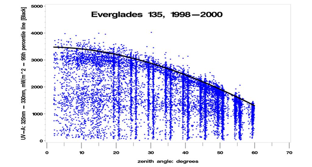
8 Atmosphere 2017, 8, of 33 to longer wavelengths, while its internal diffraction grating is physically rotated. An entire UV spectral scan, from nm to 363 nm, takes approximately six min. This yields a rate of approximately 13 nm/min of wavelength scan progression. Although Brewers are capable of measuring total column ozone, Brewer instruments in EPA s network were never initialized or calibrated to measure total column ozone. For that reason, NASA s Total Ozone Mapping Spectrometer (TOMS) satellite provided total column ozone, in Dobson Units (DUs), from its daily overpass for each of 10 sites analyzed in this study. Since only one daily satellite overpass was accomplished per site, recorded daily total column ozone values were constant for each site. The biologically damaging UV radiation is largely determined from energy in wavelengths less than 320 nm (which are very sensitive to changes in total column ozone). The effective UV wavelength band range for ozone impacts occurs at wavelengths from 290 nm to 325 nm [19]. Changes in UVR flux at wavelengths of 320 nm and greater are associated with trends in aerosols, haze, and clouds, refore wavelengths between 325 nm and 330 nm were selected to account for clouds as described below. There is less UVR sensitivity to ozone in this wavelength range. The UV spectral data scanned and recorded by Brewers between nm was used as indicator for percent clearness. This particular wavelength segment was chosen because it lies above wavelengths that are affected by total column ozone. The rational for selecting this wavelength segment ( nm) was to ensure that any changes observed could be attributed to clouds and not to any potential impacts from total column ozone. This portion of electromagnetic spectrum also provides a stable measurement basis. This wavelength segment is temporally close (within two min) to wavelength segment which provides major contribution to biologically damaging UV radiation. Given that peak biologically damaging UV radiation contribution occurs at approximately 310 nm, following calculation illustrates temporal resolution (difference) between wavelengths unaffected by total column ozone and those contributing to maximum biologically damaging UV radiation (e.g., difference between 330 nm and 310 nm is 20 nm; with an instrument scan rate of 13 nm/min: 20 nm/(13 nm/min) = min, yielding approximately 1.5 minutes temporal difference). The wavelength segment between nm was also used, which is minimally affected by clouds, to ensure that a consistent definition of cloudiness could be determined at each site using appropriate UV wavelength segment least impacted by clouds based on local site conditions. The rational for selecting this particular wavelength segment ( nm) was to attribute observed changes to total column ozone and to remove impacts from clouds. For each of 10 selected sites, a data set was generated with each observation consisting of four pieces of data including: (a) SZA measurement; (b) a total column ozone (O 3 ) measurement from TOMS; (c) a biologically damaging UV radiation (Brewer) measurement; (d) an unweighted, integrated Brewer UVR measurement taken between 325 nm and 330 nm wavelength segment (designated UV325). Using data collected at 10 selected UVR monitoring sites from 1998 through 2000, a plot of UV325 (in mw/m 2 ) versus SZA, shown in Figure 3, clearly indicates an upper envelope of UV325, which is indicative of percent clearness of sky at a given SZA. The objective is to define separate indicators for percent (sky) clearness that are unaffected by total column ozone and unaffected by clouds. Examination of UV325 versus SZA plots for 10 selected sites led to determination of CLR1 (a parameter describing a cloud free day, based on maximum range of UV irradiance values) which was added to datasets, containing (a) through (d) above, from an SZA-dependent polynomial approximation of 95th percentile of UV325 measurements for each site {as shown by black lines in Figure 3}. The polynomial regression fit for 95th percentile is: UV 95 = {cos(sza)} 3 + {cos(sza)} 2 + {cos(sza)}, (0). The parameter CLR1 is a line which represents a boundary indicating where most (95%) of UV measurements between 325 nm and 330 nm are found based on SZA at each particular site. CLR1 is parameter describing a cloud free day, according to maximum range of UV irradiance values, which would not occur on a cloudy or partially cloudy day. CLR1 tends to approach upper limit of UV325 values at each SZA, but some values can exceed CLR1 values plotted along 95th percentile line by up to 20 percent, most likely due to cloud reflections. The

9 Atmosphere 2017, 8, of 33 generated data set for each site could now be supplemented with an additional parameter (CLR1) derived from UV325 versus SZA plots: CLR1 = UV325/(95th percentile of measurements at each SZA). The ten sites selected for analysis are provided in Table 1. Brewer 105 was operated, maintained, Atmosphere 2017, and 8, 153 calibrated by Institute of Standards and Technology (NIST). Brewer 8 of was operated and maintained by US EPA. The remaining eight sites were operated, maintained, and parameter calibrated (CLR1) by derived NPS. from The graphs, UV325 residuals, versus and SZA histograms plots: CLR1 were = UV325/(95th generated using percentile SAS TM of statistical measurements software. at each SZA). The ten sites selected for analysis are provided in Table 1. Brewer 105 was operated, maintained, and calibrated by Institute of Standards and Technology (NIST). Brewer Table 087 was 1. Ten operated EPA UV Radiation and maintained Researchby Program US Sites EPA. Used The in remaining Analysis. eight sites were operated, maintained, and calibrated by NPS. The graphs, residuals, and histograms were Brewer GPS GPS Elevation Elevation Start generated using Site SAS Location Site Type Number TM statistical software. Latitude Longitude (Meters) (Feet) Date The vertical lines shown in Figure 3 are an artifact of how Brewer is configured to capture Research Triangle UV scan 087 measurement N W Urban Park (RTP), data. NC 105 Gairsburg, MD N W Urban Table 1. Ten EPA UV Radiation Research Program Sites Used in Analysis. 130 Big Bend, TX N W Brewer GPS GPS Elevation Elevation Start Park Site Location Site Type Number Great Smoky Latitude Longitude (Meters) (Feet) Date N W Research Mountains, Triangle TN Park N W Urban Park (RTP), NC 133 Canyonlands, UT N W Gairsburg, MD N W Urban Park Big Glacier, Bend, MT TX N W Park Great Smoky Park N W Park 135 Mountains, Everglades, FL TN N W Canyonlands, UT N W Park Park Shenandoah, Glacier, MT VA N W Park Park 135 Everglades, FL N W Park Shenandoah, Acadia, MEVA N W Park Park 138 Acadia, ME N W Park 144 St. John, USVI N W Park Park (a) Figure 3. Cont.

10 Atmosphere 2017, 8, of 33 Atmosphere 2017, 8, of 32 (b) (c) (d) Figure 3. Cont.

11 Atmosphere 2017, 8, of 33 Atmosphere 2017, 8, of 32 (e) (f) (g) Figure 3. Cont.

12 Atmosphere 2017, 8, of 33 Atmosphere 2017, 8, of 32 (h) (i) (j) Figure 3. Plot of UV325 versus solar zenith angle (SZA) at (a) Research Triangle Park, NC; Figure 3. Plot of UV325 versus solar zenith angle (SZA) at (a) Research Triangle Park, NC; (b) (b) Gairsburg, Gairsburg, MD; MD; (c) (c) Big Big Bend Bend Park, Park, TX; TX; (d) (d) Great Great Smoky Smoky Mountain Mountain Park, Park, TN; (e) TN; Canyonlands (e) Canyonlands Park, Park, UT; (f) UT; Glacier (f) Glacier Park, Park, MT; MT; (g) Everglades (g) Everglades Park, Park, FL; (h) FL; Shenandoah (h) Shenandoah Park, Park, VA; VA; (i) Acadia (i) Acadia Park, Park, ME; ME; (j) Virgin (j) Virgin Islands Islands Park Park (St. John), (St. John), USVI USVI (CLR1, (CLR1, illustrated illustrated by by black black line, line, represents represents polynomial polynomial of of 95th 95th percentile percentile measurement measurement at at each each SZA). SZA).

13 Atmosphere 2017, 8, of 33 The vertical lines shown in Figure 3 are an artifact of how Brewer is configured to capture UV scan measurement data Variability in Biologically Damaging UV Radiation Data It is preferable for conditions to remain constant during a scan, but that was not always case. The temporal gap between bulk of contribution to biologically damaging UV (at 310 nm) and UV325 wavelength segment introduced some variability in data. The variability appeared to be systematic, and can be illustrated through following two examples. Hypotical Situation: A day with widely scattered cumulus clouds; Example 1: At one point during day, sun is exposed (i.e., no clouds) at beginning of an instrument spectral scan. Then, at 320 nm wavelength portion of a spectral scan, a cloud passes in front of sun. The calculated UV325 will be lowered to approximately 50% of previous CLR1 value, and measured biologically damaging UV radiation value will be higher than UV325 value. Example 2: At anor point during same day, sun is hidden in early stages of a spectral scan and n emerges at approximately 320 nm, UV325 will record nearly 100% clear, and will be higher than previous CLR1 value, and measured biologically damaging UV radiation value will be lower than UV325 value. The frequency of such systematic variations tends to diminish as sky becomes eir heavily overcast (0% clear) or cloud-free (100% clear) Relationship between Biologically Damaging UV Radiation, Cloudiness, Column Ozone, and RAF Data sets were compiled for ten selected sites in UVR network containing measured parameters (SZA, total column ozone [O 3 ], biologically damaging UV radiation in erymal action spectrum, UV325), and derived CLR1 parameter. These parameters were n used to plot biologically damaging UV radiation in erymal action spectrum versus total column ozone (O 3 ), for different values of CLR1 and SZA. The biologically damaging UV radiation values were n normalized for seasonal change in Earth sun distance. Finally, although polynomials defining clear (sky) UVR are approximately same, re should be some systematic differences based on altitude, topographic obstruction, and haze/pollution at each site. For this analysis, biologically damaging UV radiation values were normalized between sites to produce a nearly identical definition of clear sky. The data from all ten sites were n combined to produce four plots shown in Figure 4 below, which display biologically damaging UV radiation in erymal action spectrum versus total column ozone (O 3 ) for percent clearness PCLR of 25% (black), 50% (blue), 75% (green), and 100% (red) ±3% and SZA from 25 to 30 degrees. The curved line relationship for RAF = 1.1 is based on power law: Biologically Damaging UV Radiation = PCLR A ((O 3 )/cos (SZA)) 1.1 (1) where A is determined from mean value of biologically damaging UV radiation for total column ozone (O 3 ), approximately 350 Dobson Units (DU). There was considerable skewing of measurements for different percentages of clearness (100% clear [red, downward]) and (50% clear [blue, upward]) as would be expected from sudden appearance or disappearance of direct sun due to cloud configuration/movement, as discussed in two hypotical examples described above. This skewing affected regression analyses designed to determine RAF oretically. Figure 4 illustrates that as total column ozone (O 3 ) increases, biologically damaging UV radiation in erymal action spectrum decreases in a consistent manner. Clouds may have a systematic effect in altering generally accepted value of a 1.1% decrease in biologically damaging UV radiation in erymal action spectrum ( 1.1%) for each 1.0% increase in total column ozone, as measured in Dobson Units (DUs).

14 Atmosphere 2017, 8, of 32 Atmosphere 2017, 8, of 33 Figure 4. The biologically damaging UV radiation versus O 3 /cos(sza) for percent clearness of 25%, Figure 4. The biologically damaging UV radiation versus O3/cos(SZA) for percent clearness of 25%, 50%, 75%, and 100% (±3%) and SZA from 25 to 30 degrees. 100% (red) light clouds; 75% (green) thin 50%, 75%, and 100% (±3%) and SZA from 25 to 30 degrees. 100% (red) light clouds; 75% (green) thin clouds; 50% (blue) moderate clouds; 25% (black) thick clouds. clouds; 50% (blue) moderate clouds; 25% (black) thick clouds Experimental Approach Used to Determine Radiation Amplification Factor (RAF) 2.6. Experimental Approach Used to Determine Radiation Amplification Factor (RAF) An initial description of relationship between cloud coverage and its effect on RAF was An initial description of relationship between cloud coverage and its effect on RAF was obtained from 71,000 total UV measurement scans taken between 1998 and 2000 at ten Brewer sites obtained from 71,000 total UV measurement scans taken between 1998 and 2000 at ten Brewer sites in EPA s UVR Monitoring Network. The range of solar zenith angles for which measurements in EPA s UVR Monitoring Network. The range of solar zenith angles for which measurements were taken was less than 60 degrees (60 were taken was less than 60 degrees (60 ). ). The relationship between biologically damaging UV The relationship between biologically damaging UV radiation, total column ozone (O radiation, total column ozone (O3), 3 ), cloudiness/percent clearness of sky, and solar zenith angle cloudiness/percent clearness of sky, and solar zenith angle was determined using experimental setup. The RAF is a parameter which is designed to answer was determined using experimental setup. The RAF is parameter which is designed to answer question, If total column ozone increases by one percent, what is percentage change in question, If total column ozone increases by one percent, what is percentage change in biologically damaging UV radiation (weighted integral of short wave UVR)? If assumption is that biologically damaging UV radiation (weighted integral of short wave UVR)? If assumption is RAF is a reasonable concept, an experiment must be designed to determine if re is a relationship that RAF is a reasonable concept, an experiment must be designed to determine if re is a between RAF and cloudiness. The idea is to isolate changes due to atmospheric ozone and relationship between RAF and cloudiness. The idea is to isolate changes due to atmospheric minimize impact of clouds when measuring changes in UVR at different wavelengths. ozone and minimize impact of clouds when measuring changes in UVR at different wavelengths Ideal Experiment 2.7. Ideal Experiment An ideal experiment to assess RAF would collect biologically damaging UV radiation An ideal experiment to assess RAF would collect biologically damaging UV radiation measurements for a period of time and would be designed as follows. For a series of fixed SZA s measurements for a period of time and would be designed as follows. For a series of fixed SZA s (e.g., (e.g., constrained between SZA = 90 degrees [ local horizon at sunrise], with SZA = 0 being directly constrained between SZA = 90 degrees [ local horizon at sunrise], with SZA = 0 being directly overhead, and SZA = 90 degrees [ local horizon at sunset]): overhead, and SZA = 90 degrees [ local horizon at sunset]): a. Measure total column ozone [O a. Measure total column ozone [O3] 3 ] levels (using eir TOMS satellite measurements or levels (using eir TOMS satellite measurements or ground measurements with spectrophotometers as applicable, etc.) at each fixed SZA. ground measurements with spectrophotometers as applicable, etc.) at each fixed SZA. b. b. Measure Measure biologically biologically damaging damaging UV UV radiation radiation levels levels (using (using ground ground measurements measurements with with spectrophotometers, spectrophotometers, etc.) etc.) at at each each fixed fixed SZA SZA at at measured: measured: i. Percent clearness = 0% [100% cloud cover] to Percent clearness = 100% [0% cloud cover]

15 Atmosphere 2017, 8, of 33 i. Percent clearness = 0% [100% cloud cover] to Percent clearness = 100% [0% cloud cover] ii. Percent clearness = 100% to 120% [accounting for cloud reflections ] Note: enhancement of UVR by cloud reflections has been measured at up to 30 percent [20], refore using a 20% enhancement (120%) for maximum biologically damaging UV radiation values provides a reasonable and conservative estimate where percent clearness (cloudiness) would be measured by satellites and/or from ground-based instruments. Total column ozone was not measured using instruments at sites, and cloudiness could not be assessed independent of human observation. The instruments could not (and cannot) measure biologically damaging UV radiation at fixed SZAs for extended periods, refore ideal experimental setup had to be adjusted to conform to limitations of real-world constraints. When developing a preliminary methodology for implementing this hyposis, an examination of initial set of UV325 versus SZA plots that were generated by statistical software indicated that clear was best defined as a SZA-dependent polynomial approximation of 95th percentile of UV325 measurements. This polynomial approximation was determined to be satisfactory, since it captured almost all of upper values, and allowed some values to exceed clear by at least 20 percent, possibly due to cloud reflections, as noted in literature [20] Realizable Experiment (Driven by Real-World Constraints) The total column ozone [O 3 ] was measured, in DUs, from TOMS satellite. The biologically damaging UV radiation is measured, in mw/m 2, from ground using Brewers. The computerized Brewer scan schedule does not accommodate measuring biologically damaging UV radiation at fixed SZAs for long periods of time. There were no independent or reliable measurements or estimates of cloud cover eir from ground-based measurements or from satellites at eir Brewer site. However, operator logs at each site recorded general sky condition and amount of cloudiness (e.g., overcast, rain, clear, sunny, etc.). This left question of how to determine percent clearness (cloudiness) unanswered. Since re was no instrument-based measurement of cloudiness (percent clearness) available at eir of Brewer sites, a oretically determined methodology for assessing percent clearness (cloudiness) was used as described below A Theoretical Definition of Cloudiness (Percent Clearness) We used wavelength segment between nm (UV325) because it is minimally affected by total column ozone, and wavelength segment between nm (UV330) which is minimally affected by clouds. This was done so that a consistent and site-appropriate definition of cloudiness was used based on local site conditions, due to differences in location, geography, climate, altitude, and ecology for each site. The polynomial representing 95th percentile of all UVA measurements, between nm, as a function of SZA is defined as 100 percent clear sky. The parameter CLR2, denoting percentage of clear sky is calculated by: Measured and Calculated Parameters CLR2 = (100 (UVA/95th percentile of UVA)) (2) The parameters used in determining RAF for each of five modeling approaches, as displayed in Figures 6, 7, 13, 16, and 17, are as follows: SZA = measured solar zenith angle of sun, where SZA = 90 degrees [ local horizon at sunrise], SZA = 0 is directly overhead, and SZA = 90 degrees [ local horizon at sunset]. O 3 = total column ozone (in Dobson Units) from TOMS satellite measurements. Biologically Damaging UV Radiation = Brewer spectrophotometer measurements.

16 Atmosphere 2017, 8, of 33 CLR2 = percent clear (percent clear sky measurement at a selected SZA) calculated value, derived from polynomial representing 95th percentile of all UVA measurements, between nm, as a function of SZA. To ensure that all potential confounding parameters are eliminated from calculation and only RAF versus percent clear curves are generated for each modeling approach, following steps were taken: a. The UVR calculations were normalized with respect to distance between sun and Earth during year. Note: Earth is closest to sun on 5 January. The formula used to calculate normalized UVR values is: UVR = { cos(2π(jday 5)/365))} Biologically Damaging UV Radiation (3) where jday = 1, 2,..., 365, with jday = 5 being 5 January, [21]. b. The UVR values were normalized with respect to systematic differences due to site altitude, topography, pollution, aerosol, haze, etc. c. The data from all ten sites was combined into curves of RAF versus percent clear sky for each of five modeling approaches, Model A through Model E, (as shown in Figures 6, 7, 13, 16, and 17 respectively). Figure 5 illustrates unweighted UVR measurements taken between nm wavelength segments. This wavelength segment is minimally affected by clouds, and is designated as UV330. The 95th percentile envelope for UV330, defined by a non-linear polynomial approximation for each site, is identical in shape to that of UV325, matching behavior of CLR1 in that wavelength segment over same SZA range, with only difference being that power values are higher for UV330 envelopes. For each of 10 selected sites, a data set was generated with each observation consisting of four pieces of data including: (a) solar zenith angle (SZA) measurement; (b) a total column ozone (O 3 ) measurement from TOMS; (c) biologically damaging UV radiation (Brewer measurement); (d) an unweighted, integrated Brewer UVR measurement taken between 330 nm and 363 nm wavelength segment (designated UV330). Using data collected at 10 selected UVR monitoring sites from 1998 through 2000, a plot of UV330 (in mw/m 2 ) versus SZA, shown in Figure 5, clearly indicates an upper envelope of UV330, which is indicative of percent clearness of sky at a given SZA. Examination of UV330 versus SZA plots for 10 selected sites led to determination of derived clear (CLR2) parameter added to datasets, (containing a through d above), from an SZA-dependent polynomial approximation of 95th percentile of UV330 measurements for each site {as shown in Figure 5}. CLR2 tends to approach upper limit of UV330 values at each SZA, but some values can exceed CLR2 values plotted along 95th percentile line by up to 20 percent, most likely due to cloud reflections. The generated data set for each site could now be supplemented with an additional parameter (CLR2) derived from UV330 versus SZA plots: CLR2 = UV330/(95th percentile of measurements at each SZA).

17 derived clear (CLR2) parameter added to datasets, (containing a through d above), from an SZA-dependent polynomial approximation of 95th percentile of UV330 measurements for each site {as shown in Figures 5}. CLR2 tends to approach upper limit of UV330 values at each SZA, but some values can exceed CLR2 values plotted along 95th percentile line by up to 20 percent, most likely due to cloud reflections. The generated data set for each site could now be supplemented Atmosphere 2017, 8, 153 with an additional parameter (CLR2) derived from UV330 versus SZA plots: CLR216 of 33 = UV330/(95th percentile of measurements at each SZA). Atmosphere 2017, 8, 153 (a) (b) (c) (d) Figure 5. Cont. 16 of 32

18 Atmosphere 2017, 8, 153 Atmosphere 2017, 8, of of 32 (e) (f) (g) Figure 5. Cont.

19 Atmosphere 2017, 8, 153 Atmosphere 2017, 8, of of 32 (h) (i) (j) Figure 5. Plot of UV330 versus SZA at (a) Research Triangle Park, NC; (b) Gairsburg, MD; (c) Big Figure 5. Plot of UV330 versus SZA at (a) Research Triangle Park, NC; (b) Gairsburg, MD; (c) Big Bend Park, TX; (d) Great Smoky Mountain Park, TN; (e) Canyonlands Bend Park, TX; (d) Great Smoky Mountain Park, TN; (e) Canyonlands Park, Park, UT; (f) Glacier Park, MT; (g) Everglades Park, FL; (h) Shenandoah UT; (f) Glacier Park, MT; (g) Everglades Park, FL; (h) Shenandoah Park, Park, VA; (i) Acadia Park, ME; (j) Virgin Islands Park (St. John), USVI (CLR2, VA; (i) Acadia Park, ME; (j) Virgin Islands Park (St. John), USVI (CLR2, illustrated illustrated by black line, represents polynomial of 95th percentile measurement at each by black line, represents polynomial of 95th percentile measurement at each SZA). SZA).

20 Atmosphere 2017, 8, of 33 The vertical lines shown in Figure 5 are an artifact of how Brewer is configured to capture UV scan measurement data. During analysis of UVR data, various parameters were kept in a limited range such as SZA, at less than 60 degrees (60 ), and wavelengths, at less than 330 nm, to ensure that only effect of clouds would manifest itself in analysis. There were five modeling approaches used in analysis of 71,000 data points analyzed between 1998 and 2000 at 10 UVR monitoring sites. Four of five modeling approaches are based on thought experiments, using empirical data, and one model is based on a purely empirical relationship (Beer Lambert s Law). The five different modeling approaches were compared to each or, and se five models each related biologically damaging UV radiation to following set of parameters (as illustrated in Table 2: Model A (1) total column ozone [O 3 ], (2) percent (%) clear sky {i.e., percent clearness/cloudiness} [CLR], (3) SZA; Model B (1) total column ozone [O 3 ], (2) clear [replaces CLR term, and is calculated by performing a regression on percentage classes of cloud cover, and result of regression is called iclear]; iclear is parameter describing cloudiness (as discrete percentage levels grouped into different classes), based on maximum range of UV irradiance values, (3) SZA; Model C (1) total column ozone [O 3 ], (2) iclear* [replaces CLR term, and is calculated by performing a regression on percentage classes of cloud cover, with removal of tails of biologically damaging UV radiation distribution, i.e., censor bad data (remove extreme values below 2.5th percentile and above 97.5th percentile), and result is called iclear*], (3) SZA Note: This is same as Model B, except with tails of biologically damaging UV radiation distribution removed; Model D (1) total column ozone [O 3 ], (2) CLRˆ [replaces CLR with a linear function in percent clearness { classes of CLR} between 40% and 100% clear skies], (3) SZA; Model E (1) total column ozone [O 3 ]/cos(sza), and (2) cos(sza): This is an empirical relationship known as Beer Lambert s Law. At 10 UVR monitoring sites selected for analysis, NASA Total Ozone Mapping Spectrometer (TOMS) satellites were used to measure total column ozone. This provided benefit of an independent measurement source for determining atmospheric (total column) ozone. Table 2. Comparison of RAF Values for Modeling Approaches Used. Model Low RAF High RAF A B C D E Functional Relationship biologically damaging UV radiation ~f (O 3, CLR, SZA) biologically damaging UV radiation ~f (O 3, iclear, SZA) biologically damaging UV radiation ~f (O 8, iclear #, SZA) with data censoring (tails of biologically damaging UV radiation distribution) biologically damaging UV radiation ~f (O 3, CLRˆ, SZA) CLR is a linear function between 40% and 100% clear skies biologically damaging UV radiation ~f (O 3 /cos[sza], cos[sza]) Calculate RAF Use Functional Relationship between Biologically Damaging UV Radiation and: total column ozone [O 3 ] CLR [percent (%) clear sky {i.e., percent clearness/cloudiness}] solar zenith angle [SZA] total column ozone [O 3 ] iclear [eliminate CLR term, and perform a regression on classes of CLR, and replace parameter CLR with result of regression on classes of clear, called iclear] solar zenith angle [SZA] total column ozone [O 3 ] revised iclear [eliminate CLR term, and perform a regression on classes of CLR, and replace parameter CLR with result of regression on classes of clear, called iclear, and remove tails of biologically damaging UV radiation distribution, i.e., censor bad data; This is same as Model B, except with tails of biologically damaging UV radiation distribution removed] solar zenith angle [SZA] total column ozone [O 3 ] CLR [assume a linear function in percent clearness { classes of CLR} between 40% and 100% clear skies] solar zenith angle [SZA] total column ozone [O 3 ]/cos(sza) cos(sza) This is known as Beer Lambert s Law

21 Atmosphere 2017, 8, of Results Each model is based on 71,000 total UVR measurements taken at ten sites listed in Table 1 between 1998 and The five modeling approaches, Model A through Model E, all yield average RAF values of approximately 1.1 for all sky conditions (e.g., 0% to 120% clear sky) at ten selected UVR monitoring sites. A consistent definition of sky cloudiness (clearness) was provided at each site using segment of UVR wavelengths least impacted by clouds (or ozone as applicable). This provided a stable baseline for comparison of each set of model-derived RAF values. Since Model E was solely based on an empirical relationship, it can be compared against four hypotical models (A through D). The summary results for each modeling approach is described below. Model A: The average RAF value from Model A for all 10 sites and for all sky conditions (i.e., in % [sky] clearness from 0% to 120%: parameter CLR) and solar zenith angles less than 60 is Model A is base model from which Models B, C, and D are derived. Model B: The average RAF value for all 10 sites and for all sky conditions and solar zenith angles less than 60 is This model performed a regression on discrete classes of parameter CLR and replaced it with result (called iclear). This model produced highest average RAF value of five models. Model C: The average RAF value for all 10 sites and for all sky conditions (i.e., in % [sky] clearness from 0% to 120%: parameter iclear*) and solar zenith angles less than 60 is This model is identical to Model B, except data censoring was applied (i.e., tails of biologically damaging UV radiation distribution [below 2.5th percentile and above 97.5th percentile] was removed). Model D: The average RAF for all 10 sites and for all sky conditions (i.e., in % [sky] clearness from 0% to 120%: parameter CLRˆ) and solar zenith angles less than 60 is The parameter representing percentage of clear sky (CLRˆ), was assumed to be a linear function between 40% and 100% clear skies. This model provided lowest average RAF value of five models. Model E: The average RAF value for all 10 sites and for all sky conditions (i.e., in % [sky] clearness from 0% to 120%) and solar zenith angles less than 60 is Model E is based on a physical/empirical model (Beer Lambert s Law). The overall average RAF value from five methods used for ten selected network sites was 1.134, with RAF values for individual methods ranging from a low of 0.80 to a high of 1.38, as shown in Table 2. The ensemble average of low RAF values resulting from five models, applied across ten selected sites, is The ensemble average of high RAF values resulting from five models, applied across ten selected sites, is The comparison of five models is presented in Table Experimental Determination of RAF: Five Modeling Approaches Model A The relationship between biologically damaging UV radiation and following parameters: (1) total column ozone [O 3 ]; (2) CLR [percent (%) clear sky {i.e., percent clearness/cloudiness}]; (3) solar zenith angle [SZA], is given as follows (where a = RAF, and b and c are regression coefficients): Biologically Damaging UV Radiation = A (O 3 ) a (CLR) b (cos(sza)) c (4) The slope of UVR ozone relationships derived for clear skies, light cloudy skies, medium cloudy skies and heavy cloudy skies for this model, can be found using formula: ln (Biologically Damaging UV Radiation) = ln (A) + a ln (O 3 ) + b ln (CLR) + c ln (cos(sza)) (5)

22 (with ln representing natural logarithm) which can be rewritten as: ln (Biologically Damaging UV Radiation) = a ln (O3) + b ln (CLR) + c ln (cos(sza)) + d Atmosphere 2017, 8, of 33 where d = ln (A), a constant. If we generate a graph of a, where a = RAF, as a function of CLR (% clearness, where 100% clear (withis lndefined representing as 95th natural percentile logarithm) of all which integrated can be UVR rewritten measurements as: for nm [where cloud effects are minimized], as a function of SZA = solar zenith angle), black line envelope in Figure 6 gives ln (Biologically 2-sigma (95%) Damaging confidence UVinterval Radiation) around = a ln value (O 3 ) + of b ln RAF. (CLR) (6) With Model A, RAF tends to increase + c ln (i.e., (cos(sza)) become + less d negative) as clear sky percentage decreases (from 45% clear sky radiation [transmitted] to 15% clear sky radiation [transmitted]). This behavior where d = is ln expected, (A), a constant. as increase in cloudiness (decrease in percent clear sky radiation transmitted) tends Ifto we reduce generate aamount graph of of a, UV where radiation a = RAF, reaching as a function Earth s of CLR surface (% for clearness, each 1% where change 100% in total clear column is defined ozone. as At 95th 45% percentile clear sky of radiation, all integrated where UVR lowest measurements RAF value for( 1.38) is found, nm [where re cloud is an inflection effects are point, minimized], after which as a function RAF values of SZA tend = solar to zenith increase angle), in general, blackwith linenegligible envelope indecreases Figure 6 (between gives 2-sigma 55% to 65% (95%) clear confidence sky radiation interval and around between 105% valueto of115% RAF. clear sky radiation). (6) % change DUV per % change ozone percent of clear sky radiation Figure Model A: RAF versus percent clear sky radiation transmitted (cloudiness) parameter (CLR) With Model Model B A, RAF tends to increase (i.e., become less negative) as clear sky percentage decreases The relationship (from 45% clear between sky radiation biologically [transmitted] damaging to 15% UV radiation clear skyand radiation following [transmitted]). parameters: This (1) behavior total column is expected, ozone as[o3]; an increase (2) iclear in cloudiness [Note: to (decrease obtain iclear, in percent replace clear sky radiation CLR term transmitted) {used in Model tends toa}, reduce with a regression amount ofperformed UV radiation on reaching classes of Earth s CLR; surface result forof each 1% regression change in on total classes column ozone. of CLR At is 45% called clear iclear ]; sky radiation, (3) solar where zenith angle lowest [SZA], RAF is given value as ( 1.38) follows: is found, re is an inflection point, after which RAF values tend to increase in general, with negligible decreases (between 55% to 65% clear Biologically sky radiation Damaging and between UV Radiation 105% to = 115% A (O3) clear a sky (CLR) radiation). b (cos(sza)) c (7) The slope of UVR ozone relationships derived for clear skies, light cloudy skies, medium cloudy Model skies B and heavy cloudy skies for this model, can be found using formula used in Model A: The relationship between biologically damaging UV radiation and following parameters: (1) total column ln (Biologically ozone [O Damaging 3 ]; (2) iclear UV Radiation) [Note: to obtain = ln (A) iclear, + a ln replace (O3) + b ln CLR (CLR) + term c {used in Model A}, with a regression performed on classes (8) ln (cos(sza)) of CLR; result of regression on classes of CLR is called iclear ]; (3) solar zenith angle [SZA], is given as follows: Biologically Damaging UV Radiation = A (O 3 ) a (CLR) b (cos(sza)) c (7) The slope of UVR ozone relationships derived for clear skies, light cloudy skies, medium cloudy skies and heavy cloudy skies for this model, can be found using formula used in Model A: ln (Biologically Damaging UV Radiation) = ln (A) + a ln (O 3 ) + b ln (CLR) + c ln (cos(sza)) (8)

23 Atmosphere 2017, 8, of of which can be rewritten in its derivative form as: which can be rewritten in its derivative form as: [δbiologically Damaging UV Radiation/δO3]/Biologically Damaging UV Radiation [δbiologically Damaging UV Radiation/δO 3 ]/Biologically Damaging UV Radiation (9) = a/(o3) + b [δclr/δo3]/clr (9) = a/(o 3 ) + b [δclr/δo3]/clr Note: The ln (A) term and c ln (cos(sza)) term both are reduced to 0 when derivatives are taken Note: since The ln (A) ln (A) is a term constant and and c cos(sza) ln (cos(sza)) is a constant, term both since are0 reduced < cos(sza) to 0 when < 1. Equation derivatives 9 can arebe reduced taken since to: ln (A) is a constant and cos(sza) is a constant, since 0 < cos(sza) < 1. Equation (9) can be reduced to: [ΔBiologically Damaging UV Radiation/Biologically Damaging UV [ Biologically Damaging UV Radiation/Biologically Damaging UV (10) Radiation]/[ΔO3/O3] = a = RAF (10) Radiation]/[ O 3 /O 3 ] = a = RAF If we generate a graph of a, where a = RAF, as a function of regression on each class of CLR If we generate graph of a, where a RAF, as a function of regression on each class of CLR (iclear where, for example, for CLR representing 40 50% clear skies, iclear = 45; for CLR (iclear where, for example, for CLR representing 40 50% clear skies, iclear = 45; for CLR representing representing % clear skies, iclear = 95%, etc.), black line envelope in Figure 7 gives % clear skies, iclear = 95%, etc.), black line envelope in Figure 7 gives 2-sigma (95%) sigma (95%) confidence interval around value of RAF. confidence interval around value of RAF. Figure 7. Model B: RAF versus percent clear sky radiation transmitted (cloudiness) parameter using classes of percent clear sky radiation transmitted (variable: iclear). With Model B, RAF tends to increase (i.e., (i.e., become less less negative) as as clear clear sky sky percentage percentage decreases (from 45% clear sky radiation [transmitted] to to 15% 15% clear clear sky sky radiation [transmitted]). This This behavioris is expected, as an increase in cloudiness (decrease in in percent clear sky sky radiation transmitted) tendsto to reduce amount of UV radiation reaching Earth s surface for for each each 1% 1% change in in total total column ozone. At 45% clear sky radiation, where lowest RAF RAF value ( 1.375) is is found, re re is is an an inflection point, after which RAF values tend to increase in in general, with aa constant region between 85% to 95% clear sky radiation and a decreasing region between 105% to to 115% clear clear sky sky radiation. The Model B residuals versus natural logarithm of of total column ozone value in in Dobson Units (LOZ), for for clear clear sky sky radiation radiation between between % % (e.g., iclear (e.g., = 95), iclear may= indicate 95), may someindicate biologically some biologically damaging UV damaging radiationuv well radiation below well expected below values expected as shown values in Figure as shown 8 below. in Figure 8 below. The Model B residuals versus natural logarithm of of total column ozone value in in Dobson Units (LOZ) for sky clearness percentages of 40 50% (iclear = 45) may indicate some biologically damaging UV radiation well above expected values, as as shown in in Figure 9 below. 9 The residuals for for sky clearness class 90% to 100% (iclear = 95), Figure 8, and for sky clearness class 40% to 50% (iclear = 45), Figure 9, would seem to indicate that Model B fits data well. But note that residuals vs LOZ for iclear = 95 seems to indicate some biologically damaging UV

24 biologically measurement damaging of spectrum UV radiation (which distributions. takes six min to complete) is a potential cause of skewed biologically The distributions damaging of UV radiation biologically distributions. damaging UV radiation as shown in Figure 11 for iclear = 45 and The iclear distributions = 95 are less of skewed, biologically and closer damaging to normality, UV radiation for this as larger shown total in Figure column 11 ozone for iclear range = as 45 compared and iclear to = 95 are total less column skewed, ozone and range closer ( to normality, DU) in for Figure this larger 10. total column ozone range as compared The distributions to total of column biologically ozone range damaging ( UV DU) radiation in Figure as shown 10. in Figure 12 are skewed in opposite The distributions directions for of iclear biologically = 45 (right) damaging and iclear UV = radiation 95 (left) for as solar shown zenith in Figure angles 12 constrained are skewed near in opposite 30 degrees. directions for iclear = 45 (right) and iclear = 95 (left) for solar zenith angles constrained near 30 degrees. Atmosphere 2017, 8, of 33 Figure 8. Model B: Residuals versus natural logarithm of total column ozone value in Dobson Figure 8. Model B: Residuals versus natural logarithm of total column ozone value in Dobson Units (LOZ) for sky clearness class 90% to 100% (iclear = 95) Note: LCZA = natural logarithm of Units cosine (LOZ) of for solar sky zenith clearness angle, class LDUV 90% = to natural 100% logarithm (iclear = 95) Note: of of biologically LCZA = natural damaging logarithm UV radiation, of cosine and LOZ of = natural solar zenith logarithm angle, of LDUV total = natural column logarithm ozone. of biologically damaging UV radiation, and LOZ = natural logarithm of total column ozone. Figure 9. Model B: Residuals versus natural logarithm of total column ozone value in Dobson Units Figure(LOZ) 9. Model for sky B: Residuals clearness versus class 40% natural to 50% (iclear logarithm = 45) Note: of total LCZA column = natural ozone logarithm value in Dobson of cosine Units (LOZ) of solar for sky zenith clearness angle, class LDUV 40% = natural to 50% (iclear logarithm = 45) Note: of biologically LCZA = damaging natural logarithm UV radiation, of and cosine LOZ of = natural solar zenith logarithm angle, of LDUV total = natural column logarithm ozone. of biologically damaging UV radiation, and LOZ = natural logarithm of total column ozone. The residuals for for sky clearness class 90% to 100% (iclear = 95), Figure 8, and for sky clearness class 40% to 50% (iclear = 45), Figure 9, would seem to indicate that Model B fits data well. But note that residuals vs. LOZ for iclear = 95 seems to indicate some biologically damaging UV radiation well below expected values. The residuals vs. LOZ for iclear = 45 may indicate some biologically damaging UV radiation well above expected values. The distributions of biologically damaging UV radiation as shown in Figure 10 are skewed in opposite directions for iclear = 45 (right) and iclear = 95 (left). Partial cloud covering during

25 Atmosphere 2017, 8, of 33 measurement of spectrum (which takes six min to complete) is a potential cause of skewed biologically damaging UV radiation distributions. Atmosphere 2017, 8, of 32 Atmosphere 2017, 8, of 32 Figure Figure Model Model B: B: The The biologically damaging UV UV radiation radiation (adjusted (adjusted for for SZA) SZA) for for 45% 45% clear clear skies skies (green) (green) and and 95% 95% clear clear skies skies (black) (black) for for total total column column ozone ozone from from Dobson Dobson Units Units (DU) (DU) to 280 to 280 DU Note: DU x-axis Note: shows x-axis shows distribution distribution of biologically of biologically damaging damaging UV radiation UV radiation wavelengths wavelengths seen seen at 45% at 45% clear clear skies (green) skies (green) and 95% and clear 95% skies clear (black) skies (black) and and y-axis y-axis shows shows percentage percentage of biologically of biologically damaging damaging UV UV radiation at each wavelength range. radiation at each wavelength range. Figure 10. Model B: The biologically damaging UV radiation (adjusted for SZA) for 45% clear skies (green) and 95% clear skies (black) for total column ozone from 250 Dobson Units (DU) to 280 DU The Note: distributions x-axis shows of distribution biologically of biologically damaging damaging UV radiation UV radiation as shown wavelengths in Figure seen at 11 45% for clear iclear = 45 and iclear skies = (green) 95 areand less 95% skewed, clear skies and (black) closer and to normality, y-axis shows for this percentage larger total of biologically column ozone damaging range as compared UV radiation to total at each column wavelength ozonerange. ( DU) in Figure 10. Figure 11. Model B: The biologically damaging UV radiation (adjusted for SZA) for 45% clear skies (green) and 95% clear skies (black) for total column ozone from 375 DU to 450 DU Note: x-axis shows distribution of biologically damaging UV radiation wavelengths seen at 45% clear skies (green) and 95% clear skies (black) and y-axis shows percentage of biologically damaging UV radiation at each wavelength range. Figure Model B: B: The The biologically damaging UV radiation (adjusted for SZA) for for 45% clear skies (green) (green) and and 95% 95% clear clear skies skies (black) for for total column ozone from 375 DUto 450 DU Note: x-axisshows shows distribution of of biologically damaging UV radiation wavelengths seenat at 45% clear skies (green) and and 95% 95% clear clear skies skies (black) and and y-axis shows percentage of biologically damaginguv UV radiationat at each each wavelength range. range.

26 Atmosphere 2017, 8, of 33 The distributions of biologically damaging UV radiation as shown in Figure 12 are skewed in opposite directions for iclear = 45 (right) and iclear = 95 (left) for solar zenith angles constrained near 30 degrees. Atmosphere 2017, 8, of 32 Figure 12. ModelB: The biologically damaging UV radiation for 45% clear skies (green) and 95% clear skies (black) for for solar zenith anglesfrom from27 27degrees degreesto to33 33 degrees Note: x-axis x-axis shows shows distribution distribution of biologically of biologically damaging damaging UV UV radiation radiation wavelengths wavelengths seen seen at 45% at 45% clear clear skies skies (green) (green) and 95% andclear 95% skies clear (black) skies (black) and and y-axis shows y-axis shows percentage percentage of biologically of biologically damaging damaging UV radiation UVat radiation each wavelength at each range. wavelength range Model Model C The The relationship between between biologically biologically damaging damaging UV UVradiation radiationand and following followingparameters: (1) (1) total column ozone [O3]; (2) iclear [Note: to obtain iclear, replace CLR term {used in 3 ]; (2) iclear [Note: to obtain iclear, replace CLR term {used in Model A}, A}, with with a a regression regression performed performed on classes on classes of CLR; of CLR; result result of regression of regression classes on classes of CLR is of called CLR iclear*, is called and iclear*, remove and remove tails of biologically tails of biologically damaging UV damaging radiationuv distribution, radiation distribution, i.e., censor bad i.e., censor data; (3) bad solar data; zenith (3) angle solar [SZA], zenith is angle identical [SZA], to Model is identical B (using to Model same B (using equations) same except equations) tails of except biologically tails of damaging biologically UV radiation damaging distributions UV radiation are distributions removed (data are censoring). removed (data If censoring). we generate a graph of a, where a = RAF, as a function of regression on each class of CLR (iclear where, If we generate for example, a graph of for a, CLR where representing a = RAF, 40 50% as a function clear skies, of iclear regression = 45; for on each CLR class representing of CLR (iclear where, % clear skies, for example, iclear = 95%, for etc.), CLR with representing data censoring 40 50% (biologically clear skies, damaging iclear = UV 45; radiation for CLR representing distribution tails % removed), clear skies, black iclear line = 95%, envelope etc.), in with Figure data 13 censoring gives (biologically 2-sigma (95%) damaging confidence UV radiation interval around distribution value tails of removed), RAF. When black line data envelope in tails in Figure of 13 biologically gives 2-sigma damaging (95%) UV confidence radiation distributions interval around are removed, value re of is minimal RAF. When effect of percent data in clear tails sky (cloudiness) of biologically on damaging RAF as compared UV radiation to Model distributions A or Model are B. removed, re is minimal effect of percent clear sky (cloudiness) With Model on C, RAF RAF as compared tends to increase to Model (i.e., A or become Model less B. negative) as clear sky percentage decreases With (from Model 25% C, clear RAF sky tends radiation to increase [transmitted] (i.e., become to 15% less clear negative) sky radiation as clear [transmitted]). sky percentage This decreases behavior is (from expected, 25% clear as an sky increase radiation in cloudiness [transmitted] (decrease to 15% in percent clear sky clear radiation sky radiation [transmitted]). transmitted) This behavior tends to reduce is expected, amount as an increase of UV radiation in cloudiness reaching (decrease Earth s in percent surface clear for sky each radiation 1% change transmitted) in total tends column to ozone. reduce Between amount 25% of and UV 45% radiation clear sky reaching radiation, re Earth s is no surface visible for change each 1% in RAF change value. in total This column ozone. Between 25% and 45% clear sky radiation, re is no visible change in RAF value. This may be a result of removal of tails of biologically damaging UV radiation distributions, which would be expected to drive values of distributions closer to mean value. This is only model without an inflection point at 45% clear sky value, which seems reasonable given censoring of tails of biologically damaging UV radiation distributions. The lowest RAF value ( 1.18) occurs at 95% clear sky radiation, which again might be attributable to

27 Atmosphere 2017, 8, of 33 may be a result of removal of tails of biologically damaging UV radiation distributions, which would be expected to drive values of distributions closer to mean value. This is Atmosphere 2017, 8, of 32 only model without an inflection point at 45% clear sky value, which seems reasonable given censoring of tails of biologically damaging UV radiation distributions. The lowest RAF value data ( 1.18) censoring occurs at used 95% clear in this skymodel. radiation, The which residuals again might for be Model attributable C censored to data data censoring are provided used in Figures in14 this and model. 15. The residuals for Model C censored data are provided in Figures 14 and 15. Figure Figure 13. Model 13. Model C: RAF C: RAF versus versus percent clear sky radiation transmitted (cloudiness) parameter parameter using using classes classes of percent of percent clear clear sky sky radiation transmitted (variable: iclear) with removal removal of tails of of tails of biologically biologically damaging UV radiation distributions. distributions. The Model The Model C residuals C residuals versus versus natural logarithm of of total total column column ozone ozone value value in Dobson in Dobson Units (LOZ) for sky clearness percentages of % (iclear = 95) indicate that biologically damaging Units (LOZ) for sky clearness percentages of % (iclear = 95) indicate that biologically damaging UV radiation mostly clusters around expected values, with a high R 2 value, as shown in Figure 14 UV radiation mostly clusters around expected values, with a high R 2 value, as shown in Figure below. The high R 2 value for Model C can be attributed to fact that extreme values were removed 14 below. by data The censoring. high R 2 The value R 2 values for Model for C residuals can be of attributed or models to are fact lower that than extreme Model values C and were removed display by data morecensoring. scatter. The R 2 values for residuals of or models are lower than Model C and display Themore Modelscatter. C residuals versus natural logarithm of total column ozone value in Dobson Units (LOZ) for sky clearness percentages of 40 50% (iclear = 45) indicate that se biologically damaging UV radiation measurements have a larger spread than those at sky clearness percentages of % (iclear = 95), with a relatively high R 2 value, as shown in Figure 15 below. At first glance, residuals for for sky clearness class 90% to 100% (iclear = 95), Figure 14, and for sky clearness class 40% to 50% (iclear = 45), Figure 15, would seem to indicate that Model C fits data well, but fact that tails of distribution were removed does not allow re to be an accurate assessment of model fit by analyzing residuals.

28 where a + b CLR^ represents a linear function in percent clearness for % clear skies. The Model C residuals versus natural logarithm of total column ozone value in Dobson Units (LOZ) for sky clearness percentages of % (iclear = 95) indicate that biologically damaging UV radiation mostly clusters around expected values, with a high R 2 value, as shown in Figure 14 below. The high R 2 value for Model C can be attributed to fact that extreme values were Atmosphere 2017, 8, of 33 removed by data censoring. The R 2 values for residuals of or models are lower than Model C and display more scatter. Atmosphere 2017, 8, of 32 Figure Figure Model Model C: C: Residuals Residuals versus versus natural natural logarithm logarithm of of total column total column ozone value ozone in Dobson value in Dobson Units (LOZ) for sky clearness class 90% to 100% (iclear = 95) with removal of tails of The Model Units C (LOZ) residuals for sky versus clearness natural class 90% logarithm to 100% (iclear of = total 95) column with removal ozone ofvalue tails in Dobson of biologically damaging UV radiation distributions Note: LCZA natural logarithm of cosine of Units (LOZ) biologically for sky damaging clearness UV percentages radiation distributions Note: of 40 50% (iclear LCZA = 45) = natural indicate logarithm that se of biologically cosine of solar solar zenith zenith angle, angle, LDUV LDUV = natural = natural logarithm logarithm of of biologically biologically damaging damaging UV radiation, UV radiation, and LOZ damaging UV radiation measurements have a larger spread than those at sky clearness percentages and = natural logarithm of total column ozone. of % LOZ = natural (iclear logarithm = 95), with of a relatively total column high ozone. R 2 value, as shown in Figure 15 below. Figure Figure Model C: C: Residuals versus natural logarithmof of total columnozone ozonevalue valuein indobson Units Units (LOZ) (LOZ) for for sky sky clearness clearness class class 40% 40% to 50% to (iclear 50% (iclear = 45) with = 45) removal with removal of tails of of tails biologically of damaging biologically UVdamaging radiationuv distributions Note: radiation distributions Note: LCZA = natural LCZA logarithm = natural logarithm of cosine of ofcosine solar of zenith solar angle, zenith LDUV angle, = natural LDUV logarithm = natural logarithm of biologically of biologically damaging damaging UV radiation, UV radiation, and LOZ and = natural LOZ logarithm = natural of logarithm totalof column total ozone. column ozone. At first glance, residuals for for sky clearness class 90% to 100% (iclear = 95), Figure 14, Model D and for sky clearness class 40% to 50% (iclear = 45), Figure 15, would seem to indicate that Model C fits The relationship data well, but between fact that biologically tails of damaging distribution UV radiation were removed and following does not allow parameters: re (1) to total be an column accurate ozone assessment [O 3 ]; (2) of model CLRˆ [assuming fit by analyzing a linear residuals. function in percent clearness { classes of CLR} for skies between 40% clear and 100% clear]; (3) solar zenith angle [SZA], is given as follows: Model D Biologically Damaging UV Radiation = A (O The relationship between biologically damaging UV 3 ) radiation a + b CLRˆ (cos(sza)) and following c (11) parameters: (1) total column ozone [O3]; (2) CLR^ [assuming a linear function in percent clearness { classes of CLR} for skies between 40% clear and 100% clear]; (3) solar zenith angle [SZA], is given as follows: Biologically Damaging UV Radiation = A (O3) a + b CLR^ (cos(sza)) c (11)

29 Atmosphere 2017, 8, of 33 where a + b CLRˆ represents a linear function in percent clearness for % clear skies. The slope of UVR ozone relationships derived for clear skies, light cloudy skies, medium cloudy skies and heavy cloudy skies for this model, can be found using formula: ln (Biologically Damaging UV Radiation) = ln(a) + a ln (O 3 ) + b CLRˆ ln (O 3 ) + c ln(cos(sza)) (12) which can be rewritten in its derivative form as: [δbiologically Damaging UV Radiation/δO 3 ]/Biologically Damaging UV Radiation = (a + b CLRˆ)/(O 3 ) (13) Note: The ln (A) term and c ln (cos(sza)) term both are reduced to 0 when derivatives are Atmosphere taken since 2017, ln 8, (A) 153 is a constant and cos(sza) is a constant, since 0 < cos(sza) < 1. Equation (13) can be 28 of 32 reduced to: [ Biologically [ΔBiologically Damaging Damaging UV Radiation/Biologically UV Radiation/Biologically Damaging Damaging UV Radiation] UV [ O Radiation] 3 /O 3 ] (14) (14) [ΔO3/O3] = (a + b = CLRˆ) (a + b = CLR^) RAF = RAF The black line envelope in Figure 16 gives 2-sigma (95%) confidence interval around The black line envelope in Figure 16 gives 2-sigma (95%) confidence interval around value value of RAF. The results were similar to those found in Model B for individual regressions using of RAF. The results were similar to those found in Model B for individual regressions using iclear* iclear* parameter parameter to represent to represent classes classes of percent of percent clearness. clearness. Note in Figure Note in 16 Figure dip 16 in RAF dip values in RAF values between between 45 55% 45 55% clearness. clearness. This couldthis indicate could isolated indicate clouds isolated passing clouds over passing sun during over individual sun during individual measurement measurement scan periods. scan periods. Figure 16. Model D: D: RAF RAF versus versus percent percent clear sky clear radiation sky radiation transmitted transmitted (cloudiness) (cloudiness) parameter (CLRˆ): parameter (CLR^): a linear a function linear function between 40% between and 100% 40% and clear100% sky radiation clear sky transmitted. radiation transmitted. With Model D, RAF tends to to increase (i.e., (i.e., become become less less negative) negative) as as clear clear sky percentage sky percentage decreases (from 45% clear sky radiation [transmitted] to to 15% 15% clear clear sky sky radiation radiation [transmitted]). [transmitted]). This This behavior is expected, as an increase in in cloudiness (decrease in in percent percent clear clear sky sky radiation radiation transmitted) tends to reduce amount of UV radiation reaching Earth s surface surface for for each each 1% change 1% change in total in total column ozone. At 45% clear sky radiation, where lowest RAF value ( 1.3) is is found, re is is an inflection an inflection point, point, after after which which RAF RAF values increase, with one exception between 85% 85 95% to 95% clear clear sky sky radiation. The RAF values between 40 60% clear sky radiation could possibly indicate an isolated cloud over sun during a scan Model E (A Model Based on an Empirical Relationship: Beer Lambert s Law)

30 Atmosphere 2017, 8, of 33 radiation. The RAF values between 40 60% clear sky radiation could possibly indicate an isolated cloud over sun during a scan Model E (A Model Based on an Empirical Relationship: Beer Lambert s Law) The functional relationship between biologically damaging UV radiation and following parameters: total column ozone [O 3 ]/cos(sza), and cos(sza), based on Beer Lambert s Law is shown in Equation (15) (where k = RAF/{O 3 /cos(sza)}): Biologically Damaging UV Radiation = A exp ( k O 3 /cos(sza)) (cos(sza)) c (15) The slope of UVR ozone relationships derived for clear skies, light cloudy skies, medium cloudy skies and heavy cloudy skies for this model, can be found using Equation (16): ln (Biologically Damaging UV Radiation) = ln (A) k O 3 /cos(sza) + c ln (cos(sza)) (16) Which can be rewritten in its derivative form as: [δbiologically Damaging UV Radiation/δO 3 ]/Biologically Damaging UV Radiation = k O 3 /cos(sza) (17) Note: The ln (A) term and c ln (cos(sza)) term both are reduced to 0 when derivatives are taken since ln (A) is a constant and cos (SZA) is a constant, since 0 < cos(sza) < 1. Equation (17) can be reduced to: [ Biologically Damaging UV Radiation/Biologically Damaging UV Radiation]/[ O 3 /O 3 ] = k O 3 /cos(sza) = RAF (18) Using fixed values for average total column ozone and average solar zenith angle facilitates sensitivity analysis of RAF. RAF = k avg O 3 /cos(avg SZA): [avg O 3 = 315 DU, avg SZA = 36 deg] (19) In order to make definition of UV-A temporally closer to definition of biologically damaging UV radiation, for this model (Model E), use UVR wavelength range of nm {UV325: Figure 3}, which is unaffected by ozone, not nm (Figure 5) used previously in Models A through D. Since empirical relationship is proportional to total column ozone, it is necessary to find portion of electromagnetic spectrum where UVR is unaffected by atmospheric ozone and observe variation of SZA and cloudiness on biologically damaging UV radiation. The black line envelope in Figure 17 gives 2-sigma (95%) confidence interval around value of RAF. Beer Lambert s Law suggests that a more suitable physical model implies that RAF is not constant but is proportional to (O 3 /cos(sza)). However, using average ozone and SZA values yielded results similar to those provided in Figure 17. Note in Figure 17 dip in RAF values between 40 50% clearness. This could indicate isolated clouds passing over sun during individual measurement scan periods. Note: There may be a relationship between seasonal ozone cycle (i.e., high ozone = spring, low ozone = fall), cloud types, and cloud coverage amounts requiring furr exploration. With Model E, RAF tends to increase (i.e., become less negative) as clear sky percentage decreases (from 45% clear sky radiation [transmitted] to 15% clear sky radiation [transmitted]). This behavior is expected, as an increase in cloudiness (decrease in percent clear sky radiation transmitted) tends to reduce amount of UV radiation reaching Earth s surface for each 1% change in total column ozone. At 45% clear sky radiation, where lowest RAF value ( 1.28) is found, re is an

31 atmospheric ozone and observe variation of SZA and cloudiness on biologically damaging UV radiation. The black line envelope in Figure 17 gives 2-sigma (95%) confidence interval around value of RAF. Beer Lambert s Law suggests that a more suitable physical model implies that RAF is not constant but is proportional to (O3/cos(SZA)). However, using average ozone and SZA values yielded results similar to those provided in Figure 17. Note in Figure 17 dip in RAF Atmosphere 2017, 8, of 33 values between 40 50% clearness. This could indicate isolated clouds passing over sun during individual measurement scan periods. Note: There may be a relationship between seasonal ozone inflection cycle (i.e., point, high ozone after = which spring, RAF low values ozone increase, = fall), cloud withtypes, exceptions and cloud between coverage 75% amounts and 85% requiring clear sky radiation, furr exploration. and between 105% and 115% clear sky radiation, consistent with [22]. Figure 17. Model E: E: RAF versus percent clear sky radiation transmitted (cloudiness) parameter: {O3/cos(SZA)/cos(SZA)}. 3 With Model E, RAF tends to increase (i.e., become less negative) as clear sky percentage Although Model A and Model B have average RAF values closer to 1.2, while Model D has an decreases (from 45% clear sky radiation [transmitted] to 15% clear sky radiation [transmitted]). This average value of nearly 1.1 ( 1.087), Model A, Model B, and Model D behave in a similar fashion, behavior is expected, as an increase in cloudiness (decrease in percent clear sky radiation transmitted) as y each display relationship where RAF decreases as clear sky increases (percent cloudiness tends to reduce amount of UV radiation reaching Earth s surface for each 1% change in total decreases) between 100% to 120% clear sky values. Each of se three models displays column ozone. At 45% clear sky radiation, where lowest RAF value ( 1.28) is found, re is an lowest RAF values ( 1.3 to 1.38) at 45% clear sky value. Due to censoring of tails of inflection point, after which RAF values increase, with exceptions between 75% and 85% clear sky biologically damaging UV radiation distribution, understandably, Model C has a flattened RAF radiation, and between 105% and 115% clear sky radiation, consistent with [22]. versus clear sky response curve. Model E, like Model A, Model B, and Model D, also has its lowest Although Model A and Model B have average RAF values closer to 1.2, while Model D has an RAF value ( 1.28) at 45% clear sky value. The average RAF value of Model E is (less average value of nearly 1.1 ( 1.087), Model A, Model B, and Model D behave in a similar fashion, as than Model A), and it displays relationship where RAF increases as clear sky increases (percent cloudiness decreases) between 85% to 105% clear sky values, unlike Models A, B, and D. 4. Conclusions This research project utilized a large dataset of UVR measurements from ten monitoring sites that were diverse with respect to spatial location, geography, climate, altitude, and ecology to calculate RAF using four hypotical approaches and one empirical model. This research project developed a consistent definition of cloudiness, independent of total column ozone, and temporally close to biologically damaging UV radiation measurements to facilitate direct and consistent comparisons between each of approaches for modeling RAF. Model C, which censors tails of biologically damaging UV radiation distribution, should not be used to assess RAF, since RAF value is artificially driven to a mean value ( 1.1). While Models A, B, and D are consistent and comparable in relationship between RAF and clear sky radiation between 100% and 120%, empirically-based model, Model E, behaves differently in that range. The results show that for all models except Model C (censored tails), in 35% to 65% range of clear sky radiation (65% to 35% cloudiness), as cloudiness decreases, RAF increases, ranging from 1.2 to 1.4, where it reaches its highest level before decreasing. Between 15% and 25% clear sky radiation (85% to 75% cloudiness), re is an increase in RAF for all models. In general, RAF tends to increase as sky conditions change from high to moderate cloudiness. Clouds block biologically damaging UV radiation in this range and behavior is qualitatively same as if stratospheric ozone was

32 Atmosphere 2017, 8, of 33 increased. UVR can experience a 4.3% increase per kilometer of altitude, from 0 km to 6.2 km, and is also affected by atmospheric pressure and aerosol density [23]. It is noted in literature that mean cloud attenuation of UVR in UV-B (wavelengths: nm) is approximately 15 30% [24]. UV radiation is also reflected by both clouds and Earth s surface [25], which complicates analyses in this area. Erymally-weighted UV-B has displayed a 3 7% decadal increase in mid and high latitudes from Nimbus 7 satellite observations [26]. For 105% to 120% clear sky radiation, RAF increases for Models A, B and E, while decreasing for Models C and D. The RAF is important because it serves as a sensitivity metric that directly relates changes in stratospheric ozone to changes in UVR flux reaching Earth s surface. Overall, resulting RAF values from five modeling approaches are consistent with those found in [27]. Acknowledgments: The author appreciates advice and guidance on this manuscript from Symielle A. Gaston and Timothy M. Barzyk from US EPA Office of Research and Development (ORD) Exposure Research Laboratory (NERL). The author gives special thanks to Jack H. Shreffler, US EPA ORD/NERL (retired), who laid foundation for this research and was an understanding mentor. Author Contributions: Eric S. Hall is solely responsible for development of this manuscript, analysis, and interpretation of results. Conflicts of Interest: The author declares no conflict of interest. The United States Environmental Protection Agency through its office of Research and Development funded and managed research described here under contract 68-D with University of Georgia at Ans (UGA); partially funded through Interagency Agreement Number DW in collaboration with Institute for Standards and Technology (NIST); partially funded through Interagency Agreement Number DW in collaboration with Oceanic and Atmospheric Administration (NOAA); and partially funded through Interagency Agreement Number DW in collaboration with Parks Service (NPS). It has been subjected to Agency review and approved for publication. Although this work was reviewed by U.S. EPA and approved for publication, it may not necessarily reflect official Agency policy. Mention of trade names or commercial products does not constitute endorsement or recommendation for use. Abbreviations CCD CFC CLR DOI DOS DU DUV EPA GMT IAG LCZA LDUV LOZ PCLR NASA NERL NIST NOAA NUVMC NPS O 3 ORD RAF SZA TOMS UGA US UV UVR charge-coupled device chlorofluorocarbon percent clear sky radiation US Department of Interior disk operating system Dobson Unit biologically damaging UV radiation US Environmental Protection Agency Greenwich Mean Time Interagency Agreement natural logarithm of cosine of solar zenith angle natural logarithm of biologically damaging UV radiation natural logarithm of total column ozone fraction of clear sky radiation Aeronautics and Space Administration EPA Exposure Research Laboratory US Institute for Standards and Technology Oceanographic and Atmospheric Administration UV Monitoring Center US Parks Service total column ozone EPA Office of Research and Development Radiation Amplification Factor Solar Zenith Angle NASA Total Ozone Mapping Spectrometer University of Georgia at Ans United States ultraviolet ultraviolet radiation

33 Atmosphere 2017, 8, of 33 References 1. Gerstl, S.A.W.; Zardecki, A.; Wiser, H.L. Biologically damaging radiation amplified by ozone depletions. Nature 1981, 294, [CrossRef] 2. Smertenko, P.; Stepanov, V.; Ol khovik, C.; Durzan, D.J. New approach to a radiation amplification factor. In Cell Biology and Instrumentation: UV Radiation, Nitric Oxide, and Cell Death in Plants; Blume, Y., Durzan, D.J., Smertenko, P., Eds.; IOS Press: Amsterdam, The Nerlands, 2006; ISBN Parisi, A.V.; Sabburg, J.; Kimlin, M.G. Scattered and Filtered Solar UV Measurements; Kluwer Academic Publishers: Dordrecht, The Nerlands, Madronich, S.; McKenzie, R.L.; Bjorn, L.O.; Caldwell, M.M. Changes in biologically active ultraviolet radiation reaching Earth s surface. J. Photochem. Photobiol. B 1998, 46, [CrossRef] 5. Pfister, G.; McKenzie, R.L.; Liley, J.B.; Thomas, A.; Forgan, B.W.; Long, C.N. Cloud coverage based on all-sky imaging and its impact on surface solar irradiance. J. Appl. Meteorol. Clim. 2003, 42, [CrossRef] 6. Hall, E.S. Ground-Based Measurement of Solar Ultraviolet Radiation. In McGraw-Hill Yearbook of Science and Technology; Kotowski, F., Jr., Ed.; McGraw-Hill Book Co.: New York, NY, USA, 2009; pp Sabburg, J. EPA/UGA, UV/QA Data Correction Project Specification (v2.3); Unpublished work, Wearhead, E.C.; Frederick, J.E. Report on Geographic and Seasonal Variability of UV Affecting Human and Ecological Health. Available online: (accessed on 17 August 2017). 9. Lenoble, J. Atmospheric Radiation Transfer; A. Deepak Publishing: Hampton, VA, USA, Warhaft, Z. An Introduction to Thermal-Fluid Engineering: The Engine and Atmosphere; Cambridge University Press: Cambridge, UK, 1997; ISBN Frederick, J.E.; Snell, H.E.; Haywood, E.K. Solar ultraviolet radiation at earth s surface. Photochem. Photobiol. 1989, 50, [CrossRef] 12. Crist, K.C.; Carmichael, G.R.; John, K. UV-B exposure and atmospheric ozone: Evaluation of radiative flux to changes in ambient ozone levels. J. Hazard. Mater. 1994, 37, [CrossRef] 13. Sivasakthivel, T.; Reddy, K.S.K. Ozone Layer Depletion and Its Effects: A Review. Available online: http: // (accessed on 17 August 2017). 14. Rowland, F.S. Stratospheric Ozone Depletion. Philos. T. Roy. Soc. B 2006, 361, [CrossRef] [PubMed] 15. McCulloch, A.; Midgley, P.M.; Ashford, P. Releases of refrigerant gases (CFC-12, HCFC-22, and HFC-134a) to atmosphere. Atmos. Environ. 2003, 37, [CrossRef] 16. United Nations Environment Programme (UNEP). The 1987 Montreal Protocol on Substances that Deplete Ozone Layer. Available online: php?sec_id=342&show_all (accessed on 17 August 2017). 17. US Environmental Protection Agency (US EPA). Clean Air Act Title VI Stratospheric Ozone Protection. 42 USC 7671 (Title 42 [The Public Health and Welfare], Chapter 85 [Air Pollution Prevention and Control], Subchapter VI [Stratospheric Ozone Protection]). Available online: (accessed on 4 August 2017). 18. Brewer MKIV Spectrophotometer Operator s Manual. Available online: grad/neubrew/docs/manuals/brewer_mkiv_service_manual.pdf (accessed on 17 August 2017). 19. Binyamin, J.; Davies, J.; McArthur, B. Validation of spectral and broadband UV-B ( nm) irradiance for Canada. Atmos. Clim. Sci. 2011, 1, [CrossRef] 20. Feister, U.; Cabrol, N.; Häder, D. UV enhancements by scattering of solar radiation from clouds. Atmosphere 2015, 6, [CrossRef] 21. ITACA. The Sun as a Source of Energy, Part 4: Irradiation Calculations. Available online: itacanet.org/-sun-as-a-source-of-energy/part-4-irradiation-calculations/ (accessed on 17 August 2017). 22. El-Nouby, A.M. Effect of stratospheric ozone in UVB solar radiation reaching Earth s surface at Qena, Egypt. Atmos. Pollut. Res. 2010, 1, [CrossRef] 23. Varotsos, C. Airborne measurements of aerosol, ozone, and solar ultraviolet irradiance in troposphere. J. Geophys. Res. Atmos. 2005, 110, [CrossRef] 24. Mckenzie, R.L.; Bjorn, L.O.; Bais, A.; Ilyas, M. Changes in biologically active ultraviolet radiation reaching Earth s surface. Photochem. Photobiol. Sci. 2003, 2, [CrossRef] [PubMed]

34 Atmosphere 2017, 8, of McKenzie, R.L.; Aucamp, P.J.; Bais, A.F.; Björn, L.O.; Ilyas, M. Changes in biologically active ultraviolet radiation reaching Earth s surface. Photochem. Photobiol. Sci. 2007, 6, [CrossRef] [PubMed] 26. Ziemke, J.R.; Chandra, S.; Herman, J.; Varotsos, C. Erymally weighted UV trends over norrn latitudes derived from Nimbus 7 TOMS measurements. J. Geophys. Res. Atmos. 2000, 105, [CrossRef] 27. Massen, F. Computing Radiation Amplification Factor RAF Using a Sudden Dip in Total Ozone Column Measured at Diekirch, Luxembourg. Available online: sudden_toc_dip.pdf (accessed on 17 August 2017) by author. Licensee MDPI, Basel, Switzerland. This article is an open access article distributed under terms and conditions of Creative Commons Attribution (CC BY) license ( View publication stats